Introduction to Portfolio Risk and Return

Mastering Portfolio Risk and Return is a foundational requirement for institutional asset managers, corporate executives, personal wealth advisors, and financial analysts seeking to optimize investment strategies across global capital markets.

Managing investment portfolios requires balancing expected financial gains against market uncertainties, a trade-off governed by quantitative principles of asset pricing, utility theory, and modern diversification.

Institutional giants such as BlackRock, which oversees approximately USD13.9 trillion in assets under management, and Vanguard rely on these quantitative frameworks to construct resilient asset allocations that mitigate downside exposure while delivering target risk-adjusted returns for millions of global investors.

This article provides an in-depth analysis of portfolio risk and return, examining major asset classes, risk aversion, mean-variance optimization, capital market lines, return generating models, the Capital Asset Pricing Model (CAPM), and risk-adjusted performance measures.

Introduction

The modern theory of portfolio management transformed financial decision-making by establishing that an asset’s risk should not be evaluated in isolation, but rather by its contribution to the overall risk and return of a diversified portfolio. Corporate treasury departments, pension funds, and sovereign wealth institutions operate in dynamic capital markets where macroeconomic volatility, interest rate shifts, and currency fluctuations continually alter investment outcomes.

Understanding Portfolio Risk and Return enables financial leaders to systematically allocate capital across asset classes, evaluate risk-reward dynamics through mathematical optimization, and quantify manager performance using standardized metrics. By combining theoretical concepts like the Capital Allocation Line (CAL) and Security Market Line (SML) with empirical market data, institutional decision-makers can navigate complex investment landscapes, maximize investor utility, and make rigorous capital budgeting decisions.

Major Asset Classes in Portfolio Construction

When forming portfolios, institutional and individual investors allocate capital across distinct major asset classes. An asset class is a group of financial securities that exhibit similar economic characteristics, trade in comparable market environments, and follow similar regulatory structures.

1. Equities

Equities represent residual ownership stakes in corporations. Investors receive returns through share price appreciation and dividend distributions. Equities generally offer high long-term real returns but exhibit substantial volatility. Leading global enterprise issuers such as Apple (holding a market capitalization exceeding USD3.2 trillion), Microsoft, and Samsung provide equity investors with capital growth tied to corporate earnings expansion and technological innovation.

2. Fixed Income

Fixed income instruments are debt securities issued by governments, municipalities, or corporations. Investors receive periodic coupon payments and the return of principal upon maturity. Fixed income securities typically offer lower expected returns than equities but provide predictable cash flows, capital preservation, and portfolio downside protection during economic contractions. Major corporate issuers include multinational firms like Toyota, alongside sovereign entities issuing U.S. Treasury obligations.

3. Cash and Cash Equivalents

Cash equivalents comprise short-term, highly liquid debt instruments such as commercial paper, treasury bills, and certificates of deposit with maturities typically under 90 days. Their primary characteristics are safety of principal, maximum liquidity, and virtually zero default risk. However, cash holdings provide low nominal returns and remain susceptible to purchasing power erosion from inflation.

4. Real Estate

Real estate encompasses physical residential, commercial, and industrial properties, as well as publicly traded Real Estate Investment Trusts (REITs). Real estate offers steady rental income, potential capital appreciation, and an effective inflation hedge. Because physical real estate carries significant transaction costs and illiquidity, institutional investors often access the asset class through liquid REIT vehicles.

5. Commodities

Commodities include physical goods such as energy products (crude oil, natural gas), industrial metals (copper, aluminum), precious metals (gold), and agricultural products. Returns depend on global supply and demand fundamentals rather than corporate earnings or interest distributions. Commodities provide substantial inflation defense and low correlation with traditional stocks and bonds.

5. Alternative Assets

Alternative investments include private equity, venture capital, hedge funds, and infrastructure investments. Institutional investors utilize alternative investments, managed by specialist firms such as Berkshire Hathaway, to capture illiquidity premiums, lower broader portfolio volatility, and generate absolute returns unattached to traditional public indexes.

—

Asset Class Comparison

Asset Class	Primary Return Source	Risk / Volatility Level	Liquidity Level	Primary Portfolio Role
Equities	Capital gains, Dividends	High	High (Public exchanges)	Growth, Capital appreciation
Fixed Income	Coupon interest, Principal repayment	Low to Moderate	High to Moderate	Income, Capital preservation
Cash Equivalents	Short-term interest	Very Low	Maximum	Liquidity, Volatility buffer
Real Estate	Rental yield, Asset appreciation	Moderate to High	Low (Physical) / High (REITs)	Income generation, Inflation hedge
Commodities	Spot price changes	High	High (Futures markets)	Inflation protection, Diversification
Alternative Assets	Capital gains, Structure yield	Very High	Very Low (Lock-up periods)	Absolute return, Alpha generation

—

Investor Risk Aversion and Utility Theory

In portfolio theory, investor behavior is modeled through utility theory, where individuals evaluate investment opportunities based on expected return and risk exposure.

Risk Attitudes

Investors are categorized into three primary risk profiles:

Risk-Averse: Demands higher expected return as compensation for accepting higher risk. A risk-averse investor will reject a fair gamble (a investment with a zero expected payoff).
Risk-Neutral: Cares solely about expected returns regardless of risk exposure.
Risk-Seeking: Accepts lower expected returns for the opportunity to engage in higher-volatility investments.

In financial economics and institutional portfolio management, investors are assumed to be rational and risk-averse.

The Mean-Variance Utility Function

To quantify investor preferences, modern portfolio theory employs the quadratic utility function:

$U = E(R) - \frac{1}{2} A \sigma^2$

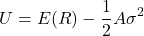
Where:

$U$ = Utility value assigned to a portfolio.
$E(R)$ = Expected return of the portfolio.
$A$ = Measure of investor risk aversion ( $A > 0$ for risk-averse investors; higher values signify greater risk aversion).
$\sigma^2$ = Variance of portfolio returns (representing total risk).

An investor’s indifference curve connects all combinations of portfolio risk ( $\sigma$ ) and expected return ( $E(R)$ ) that yield the exact same utility level ( $U$ ). For risk-averse investors, indifference curves slope upward because higher risk ( $\sigma$ ) must be compensated with higher expected returns ( $E(R)$ ). Greater risk aversion ( $A$ ) results in steeper indifference curves.

Historical Return Metrics: Mean, Variance, Covariance, and Correlation

Analyzing historical performance provides the foundation for estimating expected returns, volatility, and cross-asset relationships required for Portfolio Risk and Return modeling.

Historical Mean Return

The sample arithmetic mean return ( $\bar{R}$ ) over $n$ periods is:

$\bar{R} = \frac{1}{n} \sum_{t=1}^{n} R_t$

Sample Variance and Standard Deviation

Sample variance ( $s^2$ ) measures the dispersion of historical returns around their sample mean:

$s^2 = \frac{1}{n - 1} \sum_{t=1}^{n} (R_t - \bar{R})^2$

The sample standard deviation ( $s$ ) is the positive square root of sample variance ( $s = \sqrt{s^2}$ ).

Covariance and Correlation

Covariance ( $Cov_{A,B}$ or $\sigma_{A,B}$ ) quantifies how the returns of two assets move together:

$Cov(R_A, R_B) = \frac{1}{n - 1} \sum_{t=1}^{n} (R_{A,t} - \bar{R}_A)(R_{B,t} - \bar{R}_B)$

Correlation ( $\rho_{A,B}$ ) standardizes covariance into a scale from $-1.0$ to $+1.0$ :

$\rho_{A,B} = \frac{Cov(R_A, R_B)}{s_A \cdot s_B}$

Where $s_A$ and $s_B$ represent the standard deviations of Assets A and B.

Historical Calculation Example

Consider a 4-year historical return series for two major enterprise equities: Asset A (Apple) and Asset B (Microsoft).

Year	Asset A Return (RA)	Asset B Return (RB)	Deviation A (RA−RˉA)	Deviation B (RB−RˉB)	Product of Deviations
Year 1	15.00%	12.00%	+5.00%	+2.00%	+10.00%²
Year 2	10.00%	8.00%	0.00%	-2.00%	0.00%²
Year 3	-5.00%	2.00%	-15.00%	-8.00%	+120.00%²
Year 4	20.00%	18.00%	+10.00%	+8.00%	+80.00%²
Mean	10.00%	10.00%	0.00%	0.00%	Sum = 210.00%²

Calculating the underlying parameters ( $n = 4$ , $n - 1 = 3$ ):

Sample Variance A ( $s_A^2$ ): $(5.00^2 + 0.00^2 + (-15.00)^2 + 10.00^2) / 3 = (25 + 0 + 225 + 100) / 3 = 116.67\%^2 = 0.011667$
Standard Deviation A ( $s_A$ ): $\sqrt{116.67} = 10.801\%$
Sample Variance B ( $s_B^2$ ): $(2.00^2 + (-2.00)^2 + (-8.00)^2 + 8.00^2) / 3 = (4 + 4 + 64 + 64) / 3 = 45.333\%^2 = 0.004533$
Standard Deviation B ( $s_B$ ): $\sqrt{45.333} = 6.733\%$
Covariance ( $Cov_{A,B}$ ): $210.00 / 3 = 70.00\%^2 = 0.0070$
Correlation ( $\rho_{A,B}$ ): $70.00 / (10.8012 \cdot 6.7330) = 70.00 / 72.724 = 0.9625$

Portfolio Standard Deviation and Diversification Effects

For a two-asset portfolio with portfolio weights $w_A$ and $w_B$ (where $w_A + w_B = 1$ ), the expected return is the weighted average of individual expected returns:

$E(R_p) = w_A E(R_A) + w_B E(R_B)$

However, portfolio variance ( $\sigma_p^2$ ) depends critically on the covariance or correlation between asset returns:

$\sigma_p^2 = w_A^2 \sigma_A^2 + w_B^2 \sigma_B^2 + 2 w_A w_B Cov(R_A, R_B)$

$\sigma_p^2 = w_A^2 \sigma_A^2 + w_B^2 \sigma_B^2 + 2 w_A w_B \rho_{A,B} \sigma_A \sigma_B$

The Power of Diversification

If two assets have perfect positive correlation ( $\rho_{A,B} = +1.0$ ), portfolio standard deviation is simply the weighted average of the asset standard deviations ( $\sigma_p = w_A \sigma_A + w_B \sigma_B$ ), offering no diversification benefit.

Whenever asset returns are less than perfectly correlated ( $\rho_{A,B} < +1.0$ ), portfolio standard deviation is strictly less than the weighted average of individual standard deviations:

$\sigma_p < w_A \sigma_A + w_B \sigma_B$

If correlation is zero ( $\rho_{A,B} = 0.0$ ) or negative ( $\rho_{A,B} < 0.0$ ), portfolio risk is reduced significantly while maintaining the weighted average expected return.

Impact of Correlation on Portfolio Risk

Consider an equal-weighted portfolio ( $w_A = 0.50$ , $w_B = 0.50$ ) of Asset A ( $\sigma_A = 10.801\%$ ) and Asset B ( $\sigma_B = 6.733\%$ ), yielding an expected portfolio return $E(R_p) = 10.00\%$ .

Correlation (ρA,B)	Covariance (CovA,B)	Portfolio Variance (σp2)	Portfolio Standard Deviation (σp)	Weighted Average Risk	Volatility Reduction
+1.00 (Perfect Positive)	72.724 %²	76.861 %²	8.767%	8.767%	0.00%
+0.9625 (Historical)	70.000 %²	75.501 %²	8.689%	8.767%	0.078%
+0.20 (Low Positive)	14.545 %²	47.773 %²	6.912%	8.767%	1.855%
0.00 (Uncorrelated)	0.000 %²	40.500 %²	6.364%	8.767%	2.403%
-0.50 (Negative)	-36.362 %²	22.319 %²	4.724%	8.767%	4.043%

The Efficient Frontier and Global Minimum-Variance Portfolio

When combining multiple risky assets across different weighting schemes, investors map out the universe of achievable portfolio risk and return combinations.

The Minimum-Variance Frontier

The minimum-variance frontier represents the set of risky portfolios that offer the lowest possible variance for a given expected return level.

The Global Minimum-Variance Portfolio

The Global Minimum-Variance (GMV) portfolio sits at the leftmost tip of the minimum-variance frontier. It represents the combination of risky assets that minimizes total portfolio risk without any constraint on expected return.

The Efficient Frontier of Risky Assets

The Efficient Frontier consists of the segment of the minimum-variance frontier that lies strictly on or above the Global Minimum-Variance portfolio. Portfolios lying on the efficient frontier dominate all other portfolios of risky assets because they provide the maximum expected return for a given level of risk, or the minimum risk for a given level of expected return.

Combining a Risk-Free Asset with a Portfolio of Risky Assets

Introducing a risk-free asset (such as a short-term U.S. Treasury bill) allows investors to allocate capital between risk-free borrowing or lending and a portfolio of risky assets.

A risk-free asset has zero variance ( $\sigma_f = 0$ ) and zero covariance with all risky assets ( $Cov(R_f, R_i) = 0$ ).

When combining a risk-free asset yielding $R_f$ with a risky portfolio $i$ (having expected return $E(R_i)$ and standard deviation $\sigma_i$ ), the combined portfolio $p$ with weight $w_i$ in the risky portfolio and weight $(1 - w_i)$ in the risk-free asset yields:

$E(R_p) = (1 - w_i) R_f + w_i E(R_i) = R_f + w_i [E(R_i) - R_f]$

$\sigma_p = w_i \sigma_i \implies w_i = \frac{\sigma_p}{\sigma_i}$

The Capital Allocation Line (CAL)

Substituting $w_i = \frac{\sigma_p}{\sigma_i}$ into the expected return equation yields the Capital Allocation Line:

$E(R_p) = R_f + \left[ \frac{E(R_i) - R_f}{\sigma_i} \right] \sigma_p$

The slope of the CAL represents the Sharpe ratio of risky portfolio $i$ :

$\text{Slope of CAL} = \frac{E(R_i) - R_f}{\sigma_i}$

Investors choose the optimal risky portfolio by finding the tangency point where the CAL is tangent to the Efficient Frontier of risky assets. This tangency portfolio maximizes the slope of the CAL (the Sharpe ratio).

Capital Allocation Line (CAL) versus Capital Market Line (CML)

While the CAL applies to any arbitrary combination of a risk-free asset and a specific risky portfolio, the Capital Market Line (CML) represents a special market-wide equilibrium.

The Market Portfolio and CML

Under market equilibrium assumptions (homogenous expectations, friction-free markets), all rational investors hold the same optimal tangency portfolio of risky assets: the Market Portfolio ( $M$ ). The Market Portfolio includes all available risky assets weighted by their relative market capitalizations.

The Capital Market Line (CML) is the CAL formed by combining the risk-free asset with the Market Portfolio $M$ :

$E(R_p) = R_f + \left[ \frac{E(R_m) - R_f}{\sigma_m} \right] \sigma_p$

Where:

$E(R_m)$ = Expected return of the market portfolio.
$\sigma_m$ = Standard deviation of the market portfolio.
$\frac{E(R_m) - R_f}{\sigma_m}$ = Market price of risk.

Portfolios located on the CML are efficient portfolios composed of the risk-free asset and market portfolio $M$ . Individual securities or inefficient portfolios lie strictly below the CML because their total risk ( $\sigma$ ) contains uncompensated company-specific risk.

Systematic versus Nonsystematic Risk

Total portfolio risk can be decomposed into two distinct components:

$\text{Total Risk} = \text{Systematic Risk} + \text{Nonsystematic Risk}$

Systematic Risk (Market Risk / Non-Diversifiable Risk)

Systematic risk stems from broad macroeconomic factors that affect all market participants simultaneously, such as changes in interest rates, GDP growth, inflation, geopolitical conflicts, and tax policy. Systematic risk cannot be eliminated through portfolio diversification.

Nonsystematic Risk (Company-Specific / Diversifiable Risk)

Nonsystematic risk arises from firm-specific events, such as product recalls, management changes, labor strikes, regulatory penalties, or operational failures. Because firm-specific events are uncorrelated across different companies, holding a well-diversified portfolio (typically 30 or more assets across sectors) effectively eliminates nonsystematic risk.

Implications for Expected Return

Because rational investors can eliminate nonsystematic risk for free by holding a diversified portfolio, market prices adjust so that investors are only compensated for bearing systematic risk. No investor should expect to receive an additional return premium for holding nonsystematic risk.

Return Generating Models and Beta Analysis

Return generating models estimate the expected return of a security based on its exposure to underlying economic or market factors.

The Single-Factor Market Model

The most common return generating model is the Market Model, which expresses security returns as a linear function of a broad market index return:

$R_i = \alpha_i + \beta_i R_m + \epsilon_i$

Where:

$R_i$ = Return of asset $i$ .
$\alpha_i$ = Intercept term (asset return when market return is zero).
$\beta_i$ = Beta coefficient (sensitivity of asset $i$ to market returns).
$R_m$ = Return of the benchmark market index.
$\epsilon_i$ = Firm-specific residual error term (with an expected value of zero).

Multi-factor models (such as the Fama-French 3-factor and 5-factor models) extend this framework by incorporating additional risk drivers, including company size, value valuation multiples, profitability, and investment intensity.

Calculating and Interpreting Beta

Beta ( $\beta_i$ ) measures an asset’s systematic risk exposure relative to the aggregate market portfolio:

$\beta_i = \frac{Cov(R_i, R_m)}{\sigma_m^2} = \frac{\rho_{i,m} \cdot \sigma_i}{\sigma_m}$

$\beta = 1.0$ : The asset moves in tandem with the market (average systematic risk).
$\beta > 1.0$ : The asset exhibits above-average sensitivity to market movements (aggressive stock; e.g., tech companies).
$\beta < 1.0$ : The asset exhibits below-average sensitivity (defensive stock; e.g., consumer staple giants like Nestlé).
$\beta = 0.0$ : The asset’s return is uncorrelated with the market (e.g., risk-free Treasury bills).

The Capital Asset Pricing Model (CAPM) and Security Market Line (SML)

The Capital Asset Pricing Model (CAPM) quantifies the relationship between systematic risk ( $\beta$ ) and expected return for all assets.

Key Assumptions of CAPM

CAPM rests on several foundational assumptions:

Investors are risk-averse, utility-maximizing individuals who evaluate portfolios on a mean-variance basis.
Markets are frictionless: no taxes, transaction costs, or short-selling restrictions exist.
Investors have homogeneous expectations regarding asset returns, variances, and covariances.
All investors can borrow and lend unlimited amounts at the constant risk-free rate.
Assets are infinitely divisible and perfectly liquid.

The Capital Asset Pricing Model Equation

The fundamental CAPM equation calculates the required or expected return of asset $i$ :

$E(R_i) = R_f + \beta_i [E(R_m) - R_f]$

Where $[E(R_m) - R_f]$ is the Equity Risk Premium (ERP).

The Security Market Line (SML)

The Security Market Line (SML) is the graphical representation of CAPM. Unlike the CML (which plots expected return against total risk $\sigma$ for efficient portfolios), the SML plots expected return against systematic risk ( $\beta$ ) for all individual assets, efficient portfolios, and inefficient portfolios.

SML Y-intercept: Risk-free rate ( $R_f$ , where $\beta = 0$ ).
SML Market Point: Expected market return ( $E(R_m)$ , where $\beta = 1.0$ ).
SML Slope: Equity Risk Premium ( $E(R_m) - R_f$ ).

SML Asset Valuation Applications

Undervalued Asset: Plots above the SML. The asset provides an expected return higher than required by CAPM for its level of systematic risk. Investors buy the asset, bidding up its price and driving its expected return down toward the SML.
Overvalued Asset: Plots below the SML. The asset provides an expected return lower than required for its risk. Investors sell or short the security, causing its price to drop and raising its return back to the SML.

CAPM Calculation Example

Assume a risk-free rate ( $R_f$ ) of 4.00% and an expected market return ( $E(R_m)$ ) of 10.00% (Equity Risk Premium = 6.00%).

Apple Inc. ( $\beta = 1.09$ ):
$E(R_{\text{Apple}}) = 4.00\% + 1.09 \cdot (10.00\% - 4.00\%) = 4.00\% + 6.54\% = 10.54\%$

If an equity analyst forecasts Apple’s actual return at 11.50%, the stock is undervalued by 0.96% ( $\alpha = +0.96\%$ ), making it an attractive purchase candidate.

Risk-Adjusted Performance Measures

Evaluating investment performance requires adjusting nominal returns for the risk borne by the portfolio manager. The primary quantitative ratios used by institutional investors include the Sharpe ratio, Treynor ratio, Modigliani-Modigliani ( $M^2$ ) measure, and Jensen’s alpha.

Sharpe Ratio

The Sharpe ratio measures the excess return per unit of total risk ( $\sigma_p$ ):

$\text{Sharpe Ratio} = \frac{E(R_p) - R_f}{\sigma_p}$

It is the standard measure for evaluating non-diversified portfolios or standalone strategies.

Treynor Ratio

The Treynor ratio measures the excess return per unit of systematic risk ( $\beta_p$ ):

$\text{Treynor Ratio} = \frac{E(R_p) - R_f}{\beta_p}$

It is appropriate for evaluating fully diversified portfolios that form part of a larger asset allocation.

Modigliani-Modigliani ( $M^2$ ) Measure

The $M^2$ measure quantifies the return the portfolio would earn if it were leveraged or deleveraged to match the market portfolio’s standard deviation ( $\sigma_m$ ):

$M^2 = R_f + \left[ \frac{E(R_p) - R_f}{\sigma_p} \right] \sigma_m - E(R_m) = (\text{Sharpe}_p - \text{Sharpe}_m) \sigma_m$

$M^2$ expresses risk-adjusted performance directly as an easily interpretable percentage.

Jensen’s Alpha ( $\alpha_p$ )

Jensen’s alpha measures the abnormal return earned by a portfolio above its CAPM-predicted required return:

$\alpha_p = E(R_p) - \left[ R_f + \beta_p (E(R_m) - R_f) \right]$

A positive alpha ( $\alpha_p > 0$ ) indicates superior manager stock selection or market timing skills.

Performance Metric Application

Consider Portfolio P, Market M, and a risk-free asset:

Risk-free rate ( $R_f$ ) = 4.00%
Market Return ( $E(R_m)$ ) = 10.00%, Market Volatility ( $\sigma_m$ ) = 12.00%, Market Beta ( $\beta_m$ ) = 1.00
Portfolio P Return ( $E(R_p)$ ) = 12.00%, Portfolio Volatility ( $\sigma_p$ ) = 15.00%, Portfolio Beta ( $\beta_p$ ) = 1.20

Metric	Portfolio P Formula & Calculation	Market M Benchmark	Interpretation
Sharpe Ratio	$(12.00\% - 4.00\%) / 15.00\% = 0.5333$	$(10.00\% - 4.00\%) / 12.00\% = 0.5000$	Portfolio P generates superior excess return per unit of total risk.
Treynor Ratio	$(12.00\% - 4.00\%) / 1.20 = 6.667\%$	$(10.00\% - 4.00\%) / 1.00 = 6.000\%$	Portfolio P generates higher excess return per unit of systematic risk.
$M^2$ Measure	$4.00\% + (0.5333 \cdot 12.00\%) - 10.00\% = +0.40\%$	0.00%	Portfolio P outperforms the market benchmark by 0.40% on a total-risk-matched basis.
Jensen’s Alpha ( $\alpha_p$ )	$12.00\% - [4.00\% + 1.20 \cdot (10.00\% - 4.00\%)] = +0.80\%$	0.00%	Portfolio P generates 0.80% abnormal risk-adjusted alpha return above CAPM expectations.

Conclusions

Understanding Portfolio Risk and Return is essential for executive leadership, institutional fund managers, and financial analysts responsible for corporate capital allocation and wealth management. By systematically combining diverse asset classes—such as equities, fixed income, real estate, and alternatives—investors harvest diversification benefits that lower overall portfolio volatility without sacrificing expected financial gains.

The integration of utility theory, mean-variance optimization, and capital allocation lines enables managers to identify optimal tangency portfolios tailored to specific risk tolerances. Furthermore, the Capital Asset Pricing Model (CAPM) and Security Market Line (SML) provide robust quantitative benchmarks for valuing capital assets, evaluating systematic risk through beta, and determining hurdle rates for strategic investments.

By applying risk-adjusted evaluation metrics such as the Sharpe ratio, Treynor ratio, $M^2$ , and Jensen’s alpha, financial decision-makers ensure that institutional capital is deployed efficiently, rewarding true risk management expertise and sustainable value creation across global financial markets.

Introduction to Portfolio Risk and Return

Introduction

Major Asset Classes in Portfolio Construction

1. Equities

2. Fixed Income

3. Cash and Cash Equivalents

4. Real Estate

5. Commodities

5. Alternative Assets

Asset Class Comparison

Investor Risk Aversion and Utility Theory

Risk Attitudes

The Mean-Variance Utility Function

Historical Return Metrics: Mean, Variance, Covariance, and Correlation

Historical Mean Return

Sample Variance and Standard Deviation

Covariance and Correlation

Historical Calculation Example

Portfolio Standard Deviation and Diversification Effects

The Power of Diversification

Impact of Correlation on Portfolio Risk

The Efficient Frontier and Global Minimum-Variance Portfolio

The Minimum-Variance Frontier

The Global Minimum-Variance Portfolio

The Efficient Frontier of Risky Assets

Combining a Risk-Free Asset with a Portfolio of Risky Assets

The Capital Allocation Line (CAL)

Capital Allocation Line (CAL) versus Capital Market Line (CML)

The Market Portfolio and CML

Systematic versus Nonsystematic Risk

Systematic Risk (Market Risk / Non-Diversifiable Risk)

Nonsystematic Risk (Company-Specific / Diversifiable Risk)

Implications for Expected Return

Return Generating Models and Beta Analysis

The Single-Factor Market Model

Calculating and Interpreting Beta

The Capital Asset Pricing Model (CAPM) and Security Market Line (SML)

Key Assumptions of CAPM

The Capital Asset Pricing Model Equation

The Security Market Line (SML)

SML Asset Valuation Applications

CAPM Calculation Example

Risk-Adjusted Performance Measures

Sharpe Ratio

Treynor Ratio

Modigliani-Modigliani () Measure

Jensen’s Alpha ()

Performance Metric Application

Conclusions

Modigliani-Modigliani ( $M^2$ ) Measure

Jensen’s Alpha ( $\alpha_p$ )