Individual Asset Models - Super Business Manager

Individual Asset Models serve as the foundational analytical frameworks in modern finance, enabling corporate leaders, investment managers, and financial analysts to evaluate the intrinsic value, risk exposure, and expected cash flows of single, standalone assets.

By isolating individual assets—such as single equity shares, corporate bonds, real estate properties, energy facilities, or financial derivatives—from broad portfolio noise, Individual Asset Models provide granular insights that drive precise capital allocation, strategic mergers and acquisitions, and risk management across global markets.

Introduction: The Strategic Power of Individual Asset Models

In an increasingly complex global economy, executive teams and investment committees cannot afford to evaluate major capital expenditures or equity allocations using broad macro generalizations alone. While modern portfolio theory emphasizes diversification across asset classes, corporate value creation ultimately originates at the microeconomic level: the performance, cash flow generation, and risk characteristics of single, discrete holdings.

Individual Asset Models are mathematical, statistical, and quantitative constructs designed to appraise the risk-adjusted value of a standalone asset. Whether a financial analyst at a global investment bank is modeling an equity share, a corporate treasurer is evaluating a multi-year industrial expansion, or a private equity manager is pricing an infrastructure asset, individual asset models provide the analytical rigor required to separate intrinsic value from market speculation.

For business leaders, government advisors, and institutional investors, mastering individual asset models is essential for three primary reasons:

Precision in Capital Budgeting: Ensuring that prospective capital investments exceed their hurdle rates and generate positive net present values.
Risk Decomposition: Separating market-wide systematic risk from asset-specific unsystematic risk to determine appropriate cost of capital parameters.
Strategic Flexibility: Evaluating embedded operational options, such as the right to expand, delay, or abandon industrial projects under market uncertainty.

Theoretical Foundations of Individual Asset Valuation

The cornerstone of any individual asset model is the fundamental financial premise that the economic value of an asset equals the present value of all its expected future cash flows, discounted at a rate reflecting the asset’s inherent risk profile.

A.) Time Value of Money and Risk-Adjusted Discounting

At the core of quantitative modeling lies the Time Value of Money (TVM). Money received today possesses greater value than the same nominal amount received in the future due to its earning potential, inflation, and liquidity preference. When constructing an individual asset model, future expected cash flows ( $CF_t$ ) are discounted back to the present using an appropriate risk-adjusted discount rate ( $r$ ).

The baseline mathematical formulation for the present value ( $PV$ ) of an individual asset is expressed as:

$PV = \sum_{t=1}^{n} \frac{CF_t}{(1 + r)^t}$

Where:

$CF_t$ represents the expected net cash flow generated by the asset in period $t$ .
$r$ represents the risk-adjusted discount rate or cost of capital.
$n$ represents the total operating life or holding period of the asset.

B.) Decomposing Asset Risk: Systematic vs. Unsystematic Risk

When evaluating an individual asset, risk is bifurcated into two distinct categories:

Systematic Risk (Market Risk): Macroeconomic factors—such as interest rate shifts, inflation trends, geopolitical dynamics, and exchange rate fluctuations—that affect all assets simultaneously. Systematic risk cannot be eliminated through portfolio diversification.
Unsystematic Risk (Asset-Specific Risk): Vulnerabilities unique to the specific asset or firm, such as management decisions, operational disruptions, product liability, or supply chain bottlenecks.

Individual asset pricing models specifically quantify systematic risk to determine the expected return required by rational investors to hold that specific asset.

Primary Categories of Individual Asset Models

To address the diverse characteristics of different financial and physical assets, financial economists have developed specialized classes of individual asset models.

+-----------------------------------------------------------------------+
|                     INDIVIDUAL ASSET MODELS                           |
+-------------------+-------------------+-------------------+-----------+
|                   |                   |                   |           |
v                   v                   v                   v           
Discounted Cash     Capital Asset       Derivative & Real   Fixed Income
Flow (DCF) Models   Pricing (CAPM)      Options Models      & Debt Models

1.) Discounted Cash Flow (DCF) Models for Equity and Enterprise Valuation

The Discounted Cash Flow model remains the benchmark valuation tool for equity shares and capital investments. DCF models evaluate an asset based on its capacity to generate unencumbered cash for capital providers.

Free Cash Flow to Firm (FCFF) Framework

For individual operating assets or entire corporations, analysts calculate Free Cash Flow to Firm, which represents the cash available to all equity and debt holders after operating expenses, taxes, working capital investments, and capital expenditures (CapEx) are accounted for:

$FCFF = EBIT \times (1 - T) + D\&A - \Delta NWC - CapEx$

Where $EBIT$ is Earnings Before Interest and Taxes, $T$ is the effective marginal tax rate, $D\&A$ represents Depreciation and Amortization, $\Delta NWC$ is the change in Net Working Capital, and $CapEx$ is Capital Expenditures.

Terminal Value Estimation

Because operating assets often possess infinite or extended lifetimes, individual asset models split valuation into a discrete forecast horizon (typically 5 to 10 years) and a Terminal Value ( $TV$ ). The Terminal Value is calculated using the Gordon Growth Model:

$TV_n = \frac{FCFF_{n+1}}{WACC - g}$

Where $WACC$ is the Weighted Average Cost of Capital and $g$ is the perpetual long-term growth rate of the asset’s cash flows. Combining discrete cash flows and terminal value yields the overall asset value:

$PV = \sum_{t=1}^{n} \frac{FCFF_t}{(1 + WACC)^t} + \frac{TV_n}{(1 + WACC)^n}$

Real-world equity analysts frequently apply this individual asset model to mega-cap enterprise entities such as Apple Inc., whose market capitalization surpassed USD4.90 trillion in 2026. By projecting Apple Inc.‘s ecosystem hardware sales and high-margin recurring services cash flows, analysts model the equity share as an individual income-generating asset.

2.) Single-Factor and Capital Asset Pricing Models (CAPM)

While DCF models focus on intrinsic cash flow generation, risk-return asset models determine the required rate of return for an individual asset based on its sensitivity to global markets.

The Capital Asset Pricing Model (CAPM)

Formulated by William Sharpe, the CAPM calculates the expected rate of return $E(R_i)$ for an individual asset $i$ relative to market risk:

$E(R_i) = R_f + \beta_i \left( E(R_m) - R_f \right)$

Where:

$R_f$ is the risk-free rate of return (typically benchmarked against 10-year US Treasury yields).
$\beta_i$ (Beta) is the individual asset’s covariance with the market portfolio divided by the variance of the market portfolio ( $\beta_i = \frac{Cov(R_i, R_m)}{Var(R_m)}$ ).
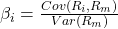$E(R_m) - R_f$ is the Market Risk Premium (MRP).

An asset with a $\beta_i > 1.0$ exhibits higher volatility than the overall market, requiring a higher return premium. Conversely, an asset with $\beta_i < 1.0$ displays lower market sensitivity.

Single-Index Asset Model

To simplify full covariance modeling across thousands of security pairs, William Sharpe introduced the Single-Index Model, which assumes an individual asset’s return is driven by a single macroeconomic market factor plus an asset-specific residual component:

$R_{i,t} = \alpha_i + \beta_i R_{m,t} + \epsilon_{i,t}$

Where $\alpha_i$ represents the asset’s excess return (alpha), $R_{m,t}$ is the market index return, and $\epsilon_{i,t}$ is the zero-mean random error term representing firm-specific unsystematic risk.

3.) Option Pricing and Real Options Individual Asset Models

Certain individual assets contain non-linear, contingent payoff structures that linear valuation tools like standard DCF or CAPM cannot capture. These include traded options, warrants, convertibles, and physical capital investments with embedded strategic flexibility.

The Black-Scholes-Merton Option Model

The Black-Scholes-Merton model provides a closed-form analytical solution for European call and put options on individual underlying assets:

$C(S_0, t) = S_0 N(d_1) - K e^{-r(T-t)} N(d_2)$

Where the parameters $d_1$ and $d_2$ are defined as:

$d_1 = \frac{\ln(S_0 / K) + \left( r + \frac{\sigma^2}{2} \right)(T - t)}{\sigma \sqrt{T - t}}$

$d_2 = d_1 - \sigma \sqrt{T - t}$

In this formulation, $S_0$ is the current spot price of the individual asset, $K$ is the strike price, $r$ is the risk-free interest rate, $T - t$ is time to maturity, $\sigma$ is the annualized volatility of the underlying asset, and $N(\cdot)$ is the cumulative standard normal distribution function.

Real Options in Corporate Asset Management

In industrial corporate settings, executives evaluate high-risk projects—such as greenfield oil drilling fields at Saudi Aramco or AI data center construction at Microsoft Corporation—using Real Options analysis. Real Options adapt financial option pricing models to value managerial choices to defer, expand, contract, or abandon physical asset developments as market conditions unfold.

4.) Fixed Income and Debt Individual Asset Models

Individual debt assets, such as corporate bonds, sovereign debt securities, and commercial loans, possess fixed or floating contractual cash flows and defined maturity dates.

Bond Cash Flow Discounting and Yield-to-Maturity (YTM)

The price ( $P_0$ ) of a traditional individual fixed-rate bond with face value ( $F$ ), annual coupon payment ( $C$ ), and $N$ periods to maturity is modeled as:

$P_0 = \sum_{t=1}^{N} \frac{C}{(1 + y)^t} + \frac{F}{(1 + y)^N}$

Where $y$ represents the Yield-to-Maturity (YTM)—the internal rate of return earned by an investor purchasing the debt asset at price $P_0$ and holding it until final maturity.

Macaulay and Modified Duration

To measure an individual debt asset’s price sensitivity to changing interest rates, analysts calculate Modified Duration ( $D_{mod}$ ):

$D_{mac} = \frac{\sum_{t=1}^{N} \frac{t \cdot C}{(1 + y)^t} + \frac{N \cdot F}{(1 + y)^N}}{P_0}$

$D_{mod} = \frac{D_{mac}}{1 + \frac{y}{m}}$

Where $m$ is the coupon payment frequency per year. A higher duration indicates greater price volatility in response to benchmark yield fluctuations.

5.) Real Estate and Infrastructure Individual Asset Models

Physical real estate assets and infrastructure networks require specialized individual valuation models focused on localized market supply, tenant creditworthiness, operational expenditures, and capitalization rates.

Net Operating Income (NOI) and Capitalization Rate Model

In commercial real estate modeling, property value ( $V$ ) is determined by dividing expected annual Net Operating Income ( $NOI$ ) by the prevailing market Capitalization Rate ( $R_{cap}$ ):

$NOI = Gross\ Potential\ Income - Vacancy\ \&\ Credit\ Losses - Operating\ Expenses$

$V = \frac{NOI}{R_{cap}}$

Luxury multi-brand conglomerates such as LVMH apply rigorous single-asset real estate models when acquiring prime commercial properties on Avenue des Champs-Élysées in Paris or Fifth Avenue in New York. For LVMH, purchasing flagship real estate assets shields the conglomerate from long-term retail rent inflation while securing strategic distribution locations for its prestige brands.

Comprehensive Comparative Matrix of Individual Asset Models

To assist chief financial officers, investment analysts, and corporate strategists in selecting the appropriate analytical tool, the following comparative matrix synthesizes the primary individual asset models:

Model Name	Primary Asset Class	Key Input Variables	Core Outputs	Major Strengths	Primary Limitations
Discounted Cash Flow (DCF)	Equities, Capital Projects, M&A	Expected Cash Flows ( $CF$ ), WACC, Terminal Growth Rate ( $g$ )	Net Present Value (NPV), Intrinsic Equity Value	Focuses on intrinsic cash generation; highly adaptable	Sensitive to growth and discount rate assumptions
Capital Asset Pricing Model (CAPM)	Publicly Traded Equities	Risk-Free Rate ( $R_f$ ), Beta ( $\beta$ ), Market Return ( $E(R_m)$ )	Required Rate of Return, Cost of Equity	Standardizes risk-adjusted required return; simple to compute	Assumes linear market risk; ignores firm-specific tail risks
Single-Index Model	Traded Securities	Stock Returns, Market Index Returns, Historical Covariance	Asset Beta ( $\beta_i$ ), Alpha ( $\alpha_i$ ), Residual Risk	Drastically reduces parameter estimation in covariance matrices	Assumes single macro factor drives all systematic volatility
Black-Scholes-Merton	Financial Derivatives, Options	Spot Price ( $S$ ), Strike ( $K$ ), Volatility ( $\sigma$ ), Rate ( $r$ ), Time ( $T$ )	Option Fair Price, Greeks ( $\Delta, \Gamma, \Theta, \ Vega$ )	Analytical precision for European contingent payoffs	Assumes constant volatility and continuous trading
Real Options Valuation	Strategic Industrial Assets	Project Capital Cost, Volatility of Underlying Demand, Time Window	Strategic NPV, Optimal Execution Threshold	Quantifies managerial flexibility and operational choices	High mathematical complexity; subjective parameter estimation
Yield-to-Maturity & Duration	Bonds, Fixed Income Debt	Coupon Payment ( $C$ ), Face Value ( $F$ ), Market Price ( $P$ ), Maturity ( $N$ )	YTM, Macaulay/Modified Duration	Clear contractual focus; precise interest rate risk metric	Assumes reinvestment at constant YTM; poor for callable bonds
Cap Rate Model	Commercial Real Estate	Gross Revenue, Operating Expenses, Market Cap Rate ( $R_{cap}$ )	Property Asset Value ( $V$ )	Rapid property comparisons; reflective of localized yield	Ignores multi-year cash flow trajectories and debt structures

Strategic Real-World Corporate Applications and Case Studies

To understand how Individual Asset Models function in real-world corporate governance and global capital markets, we examine four global corporate applications across distinct industrial sectors.

Corporate Case Study 1: Equity Asset Valuation at Apple Inc.

In public equity valuation, global investment institutions treat shares of Apple Inc. as single equity assets evaluated through multi-stage DCF models.

Suppose an analyst models an equity share of Apple Inc. using a two-stage FCFF framework. The analyst establishes the following parameter assumptions:

Current Free Cash Flow to Firm ( $FCFF_0$ ): USD108 billion.
Forecast Stage 1 (Years 1 to 5): Annual FCFF growth rate of 7.5% driven by services sector expansion and ecosystem monetization.
Forecast Stage 2 (Perpetual Growth $g$ ): 3.0% long-term growth rate.
Risk-Free Rate ( $R_f$ ): 4.25% (US 10-Year Treasury Bond Yield).
Asset Beta ( $\beta_{Apple}$ ): 1.08.
Equity Market Risk Premium ( $MRP$ ): 5.00%.

Using CAPM to establish the required Cost of Equity ( $r_e$ ):

$r_e = 4.25\% + 1.08 \times 5.00\% = 4.25\% + 5.40\% = 9.65\%$

Assuming an overall corporate WACC of 9.20% (reflecting Apple Inc.‘s low-cost corporate bond issuances), the analyst projects the cash flow stream:

Year 1: $USD108.00\text{ bn} \times 1.075 = USD116.10\text{ bn}$
Year 2: $USD116.10\text{ bn} \times 1.075 = USD124.81\text{ bn}$
Year 3: $USD124.81\text{ bn} \times 1.075 = USD134.17\text{ bn}$
Year 4: $USD134.17\text{ bn} \times 1.075 = USD144.23\text{ bn}$
Year 5: $USD144.23\text{ bn} \times 1.075 = USD155.05\text{ bn}$

Calculating the Terminal Value at Year 5:

$TV_5 = \frac{USD155.05\text{ bn} \times (1 + 0.030)}{0.092 - 0.030} = \frac{USD159.70\text{ bn}}{0.062} = USD2,575.81\text{ bn}$

Discounting all cash flows and the terminal value back to Present Value at WACC = 9.20%:

$PV(FCFF_{1-5}) = \frac{116.10}{1.092^1} + \frac{124.81}{1.092^2} + \frac{134.17}{1.092^3} + \frac{144.23}{1.092^4} + \frac{155.05}{1.092^5} = USD508.83\text{ bn}$

$PV(TV_5) = \frac{USD2,575.81\text{ bn}}{1.092^5} = USD1,658.89\text{ bn}$

$Total\ Enterprise\ Value = USD508.83\text{ bn} + USD1,658.89\text{ bn} = USD2,167.72\text{ bn}$

Adjusting for net cash holdings yields the final equity value. This single-asset equity model allows portfolio managers to continuously monitor whether current market pricing offers a sufficient margin of safety.

Corporate Case Study 2: Capital Budgeting for EV Production Facilities at Toyota Motor Corporation

When corporate executives at Toyota Motor Corporation decide whether to construct a dedicated electric vehicle (EV) battery assembly facility, they treat the proposed plant as an individual physical asset model.

Suppose Toyota Motor Corporation evaluates a facility with the following financial parameters:

Initial Capital Investment ( $CapEx$ ): USD1.50 billion.
Useful Asset Life: 10 years.
Expected Annual Operating Cash Flow ( $CF_t$ ): USD280 million.
Salvage Value at Year 10: USD200 million.
Corporate Hurdle Rate (WACC): 8.00%.

The Net Present Value (NPV) calculation is structured as:

$NPV = -USD1,500\text{ million} + \sum_{t=1}^{10} \frac{USD280\text{ million}}{(1.08)^t} + \frac{USD200\text{ million}}{(1.08)^{10}}$

Calculating the Present Value of the 10-year annuity:

$PV(Annuity) = USD280\text{ million} \times \left[ \frac{1 - (1.08)^{-10}}{0.08} \right] = USD280\text{ million} \times 6.7101 = USD1,878.83\text{ million}$

Calculating the Present Value of the Salvage Value:

$PV(Salvage) = \frac{USD200\text{ million}}{(1.08)^{10}} = \frac{USD200\text{ million}}{2.1589} = USD92.64\text{ million}$

Summing the present values yields:

$NPV = -USD1,500\text{ million} + USD1,878.83\text{ million} + USD92.64\text{ million} = +USD471.47\text{ million}$

Because the NPV is significantly positive (+USD471.47 million), Toyota Motor Corporation‘s management receives a clear financial signal that allocating capital to this individual manufacturing asset will enhance overall shareholder value.

Corporate Case Study 3: Megaproject Real Options Modeling at Saudi Aramco

In capital-intensive sector energy production, state-backed energy titan Saudi Aramco evaluates offshore oil fields where energy price volatility presents both downside risk and upside opportunity. Traditional static DCF models often penalize such projects due to high upfront risk discount rates.

By employing a Real Options Individual Asset Model (using Black-Scholes or Binomial Trees), Saudi Aramco models the investment as a European Call Option:

Underlying Asset Value ( $S_0$ ): Present value of oil reserves expected from the field at current crude oil spot prices = USD5.00 billion.
Strike Price ( $K$ ): Capital expenditure required to construct offshore extraction platforms = USD5.20 billion.
Time to Option Expiry ( $T$ ): 3 years (the period during which Saudi Aramco holds exclusive exploration licenses before commencing construction).
Risk-Free Rate ( $r$ ): 4.00%.
Volatilty of Oil Prices ( $\sigma$ ): 35.00% annually.

While a static DCF model indicates a negative NPV ( $USD5.00\text{ bn} - USD5.20\text{ bn} = -USD200\text{ million}$ ), the Real Options model yields a positive option value due to high commodity volatility ( $\sigma = 35\%$ ). The option to delay construction for up to 3 years allows Saudi Aramco to preserve capital if crude prices decline, while retaining the right to execute the megaproject if market prices surge.

Corporate Case Study 4: Commercial Real Estate Single-Asset Valuation at LVMH

When luxury group LVMH evaluates prime commercial real estate acquisitions for its retail portfolio, investment managers deploy single-asset real estate income models.

Suppose LVMH considers acquiring a flagship retail property with the following metrics:

Gross Potential Rental Income: USD35.00 million per year.
Vacancy and Bad Debt Allowance: 4.00%.
Annual Property Operating Expenses (Taxes, Insurance, Maintenance): USD6.40 million.
Prevailing Commercial Capitalization Rate ( $R_{cap}$ ): 4.25%.

Step 1: Calculate Net Operating Income (NOI):

$Effective\ Gross\ Income = USD35.00\text{ million} \times (1 - 0.04) = USD33.60\text{ million}$

$NOI = USD33.60\text{ million} - USD6.40\text{ million} = USD27.20\text{ million}$

Step 2: Calculate Implied Single-Asset Valuation ( $V$ ):

$V = \frac{USD27.20\text{ million}}{0.0425} = USD640.00\text{ million}$

This direct capitalization asset model provides LVMH‘s real estate investment committee with a benchmark valuation of USD640.00 million, establishing the upper limit for purchase negotiations.

Advanced Sensitivity Analysis and Quantitative Enhancements

Static individual asset models rely on fixed input parameters. However, in volatile macroeconomic environments, individual asset performance is subject to uncertainty. To enhance decision-making, quantitative analysts integrate advanced simulation techniques.

+-----------------------------------------------------------------------+
|                    QUANTITATIVE ENHANCEMENTS                          |
+-------------------+-------------------+-------------------------------+
|                   |                   |                               |
v                   v                   v                               
Monte Carlo         Macro Stress        Parameter Optimization          
Simulations         Testing             & Data Aggregation              
(10,000+ Iterations) (Interest/FX Shifts)(Sensitivities & Calibration)

Monte Carlo Simulations in Individual Asset Models

Rather than calculating a single deterministic Net Present Value, analysts run Monte Carlo simulations across individual asset models. By defining probability distributions for key uncertain parameters—such as revenue growth rates, raw material costs, and interest rates—a computer algorithm executes 10,000 or more iterations of the model.

The resulting output generates a probability distribution of asset outcomes, displaying:

Expected Value (Mean NPV).
Value at Risk (VaR): The minimum expected loss at a specified confidence level (e.g., 95% 1-year VaR).
Probability of Loss: The likelihood that the asset’s NPV falls below USD0.

Macroeconomic Stress Testing

To ensure individual assets remain resilient during economic shocks, stress testing evaluates asset cash flows under extreme scenarios:

Interest Rate Spikes: Assessing the impact of a +200 basis point shift in central bank policy rates on debt service coverage ratios and discount rates.
Foreign Exchange Volatility: Testing cash flows for assets operating in emerging markets against rapid currency depreciations.
Input Cost Inflation: Simulating a 20% surge in energy or raw material costs to test corporate profit margins.

Implementation Framework for Business Leaders and Investment Managers

To successfully execute and maintain robust individual asset models within an organization, executive leadership should implement a standardized four-stage operational framework:

Stage 1: Parameter Definition & Data Aggregation
  │
  ▼
Stage 2: Model Architecture Construction & Verification
  │
  ▼
Stage 3: Sensitivity, Scenario & Monte Carlo Testing
  │
  ▼
Stage 4: Operational Governance & Continuous Audit

Parameter Definition & Data Aggregation: Establish rigorous protocols for sourcing input data. Financial metrics must be verified against audited financial disclosures, market feeds, and macroeconomic data.
Model Architecture Construction & Verification: Build standardized valuation models with clear separation between inputs, calculation engines, and summary dashboards. Perform mathematical checks to confirm formula accuracy and balance sheet integrity.
Sensitivity, Scenario & Monte Carlo Testing: Conduct comprehensive sensitivity analysis on critical drivers (such as hurdle rates, unit sales, and terminal growth values). Stress test the asset under adverse economic conditions.
Operational Governance & Continuous Audit: Establish model governance procedures. Periodically audit historical individual asset model forecasts against actual operational performance to refine parameter assumptions over time.

Conclusion: Navigating Future Trends in Individual Asset Valuation

Individual Asset Models remain essential instruments for rigorous financial analysis, capital budgeting, and asset pricing. By providing clear frameworks to evaluate standalone investments, these models empower CEOs, managers, institutional investors, and policymakers to make capital allocation decisions grounded in economic reality rather than speculative impulse.

Looking ahead, the evolution of individual asset modeling will be shaped by three major technological and economic developments:

Integration of Artificial Intelligence and Machine Learning: Automated data pipelines will dynamically adjust individual asset model inputs in real time, incorporating high-frequency satellite data, supply chain tracking, and live market sentiment.
Environmental, Social, and Governance (ESG) Parameterization: Valuations will increasingly incorporate climate risk adjustments, carbon pricing costs, and regulatory compliance liabilities directly into individual asset discount rates and cash flow forecasts.
Real-Time Private Market Valuation Platforms: As private equity and private credit asset classes continue to expand, institutional managers will increasingly replace static spreadsheet modeling with continuous individual asset tracking platforms.

Organizations that master individual asset models—combining rigorous financial theory with quantitative stress testing and real-world corporate data—will maintain a distinct competitive advantage in allocating capital, managing risk, and creating sustainable long-term value.