Applications of Simple Linear Regression in Finance

Understanding the applications of simple linear regression in finance provides corporate executives, portfolio managers, quantitative analysts, and financial advisors with a rigorous quantitative framework for data-driven decision-making.

Simple linear regression is a fundamental econometric technique designed to model and evaluate the functional relationship between a single independent variable () and a continuous dependent variable ().

Within capital markets, quantitative risk management, and corporate finance, this model allows practitioners to estimate asset pricing parameters, calculate cost of capital, measure systemic market risk, forecast earnings, assess corporate debt default probabilities, and conduct robust statistical hypothesis testing.

By fitting an optimal straight line through historical empirical data via the Ordinary Least Squares (OLS) criterion, financial decision-makers extract actionable parameters that govern asset valuations and strategic capital allocations.

Theoretical Foundations and Ordinary Least Squares Estimation

Simple linear regression models the true population relationship between a scalar dependent financial outcome () and an explanatory independent driver (). In econometric theory, the population regression function is defined as:

Where:

• represents the dependent financial variable (such as equity return, portfolio loss rate, sales volume, or corporate bond yield).
• represents the independent explanatory variable (such as benchmark index return, marketing spend, interest rate shift, or credit score).
• represents the true population intercept coefficient, indicating the expected baseline value of when .
• represents the true population slope coefficient, quantifying the directional sensitivity and expected magnitude of change in for every one-unit change in .
• represents the unobservable random error term (residual shock), capturing exogenous noise, measurement inaccuracies, and omitted structural drivers.

Because true population parameters ( and ) are unobservable, analysts compute sample estimates ( and ) using historical observations, resulting in the sample regression function:

Where is the fitted or predicted value of , and the sample residual is .

The Least Squares Criterion and Mathematical Derivation

The Ordinary Least Squares (OLS) estimation technique derives sample coefficients by minimizing the Sum of Squared Errors (), defined as the sum of squared differences between actual observed values () and fitted regression estimates ():

To find the minimum, partial derivatives of are taken with respect to and and set equal to zero, yielding the first-order normal equations:

Solving these equations simultaneously yields the closed-form formulas for coefficient estimation:

Where and represent the sample arithmetic means of the independent and dependent variables, respectively.

Interpretation of Regression Parameters in Business Settings

To illustrate parameter interpretation, consider consumer goods leader Unilever PLC. Corporate finance teams regress quarterly gross revenues (, in USD Millions) against global marketing expenditure (, in USD Millions).

If Ordinary Least Squares estimation yields and , financial managers interpret these coefficients as follows:

• Intercept (): In the hypothetical absence of quarterly brand marketing expenditure (), baseline consolidated revenue is estimated at USD8,500 million, driven by organic retail presence and brand equity.
• Slope (): For every incremental USD1.00 million increase in advertising spend, gross revenue increases by an expected average of USD3.40 million.

Econometric Assumptions, Residual Analysis, and Model Diagnostics

The validity of classical statistical inference (such as hypothesis testing and confidence interval estimation) relies on four critical Gauss-Markov assumptions regarding the regression model and its unobserved error terms ().

Classical Assumptions of Simple Linear Regression

1. Linearity in Parameters: The relationship between the dependent variable and independent variable is linear in parameters.
2. Exogeneity / Zero Conditional Mean of Errors: The expected value of error terms conditional on is zero ().
3. Homoscedasticity (Constant Error Variance): The variance of the error term is constant across all observations of ().
4. No Autocorrelation (Independence of Errors): Error terms associated with different observations are uncorrelated ( for ).
5. Normality of Errors: Error terms are normally distributed (), essential for exact small-sample hypothesis testing.

Residual Analysis and Identification of Model Violations

Residual analysis involves plotting sample residuals () against fitted values () or time periods to visually and statistically detect underlying model violations.

Econometric Assumption Violation	Underlying Cause in Financial Data	Visual Residual Pattern	Statistical Test	Impact on Estimation & Inference	Financial Mitigation Remedy
Heteroscedasticity	Volatility clustering during financial crises; variance expands as market caps grow.	Fan-shaped or funnel-shaped residual distribution.	Breusch-Pagan Test; White Test	OLS estimates remain unbiased, but standard errors are wrong, invalidating -tests.	Use White’s heteroscedasticity-consistent (robust) standard errors; transform variables.
Autocorrelation (Serial Correlation)	Economic time-series exhibit momentum, persistent inflation, or interest rate trends.	Cyclical, wave-like residual patterns over consecutive time periods.	Durbin-Watson Statistic (); Breusch-Godfrey Test	Standard errors are understated, leading to falsely high -statistics and false significance.	Implement Newey-West HAC standard errors; apply autoregressive lag models.
Non-Normality of Residuals	Asset returns feature fat tails (leptokurtosis) and extreme sudden crashes.	Significant departure from straight line on Normal Q-Q plot.	Jarque-Bera Test; Shapiro-Wilk Test	Distorts exact confidence intervals and critical rejection regions in small samples.	Increase sample size ; apply non-parametric methods or logarithmic transformations.
Omitted Variable Bias	Regressing returns on only one market factor while ignoring interest rates/inflation.	Systematic non-linear curvature in residual scatter plots.	Ramsey RESET Test	Coefficient estimates become biased and inconsistent.	Expand to multiple linear regression models (e.g., multi-factor asset pricing).

Evaluating Goodness-of-Fit, ANOVA Estimates, and Hypothesis Testing

Evaluating an estimated regression model requires decomposing total variation into explained and unexplained components using Analysis of Variance (ANOVA).

ANOVA Decomposition of Variation

Total variation in the dependent variable around its mean is measured by the Total Sum of Squares (), which decomposes into the Regression Sum of Squares () and the Sum of Squared Errors ():

Where:

• Total Sum of Squares (): Total variation of around its sample mean ( degrees of freedom).
• Regression Sum of Squares (): Variation explained by the linear regression line ( degree of freedom).
• Sum of Squared Errors (): Unexplained residual variation ( degrees of freedom).

Source of Variation	Sum of Squares (SS)	Degrees of Freedom (df)	Mean Square (MS)	F-Statistic Formula
Regression (Explained)
Error (Unexplained)				—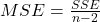
Total			—	—

Goodness-of-Fit: Coefficient of Determination () and Standard Error of the Estimate ()

The Coefficient of Determination () measures the proportion of total variation in that is explained by the independent variable :

In simple linear regression, equals the square of the sample Pearson correlation coefficient (). An of 0.65 indicates that 65% of the variance in the dependent variable is explained by the linear relationship with .

The Standard Error of the Estimate (), also known as the standard error of the residual, measures the model’s prediction precision:

A smaller indicates tighter clustering of empirical data points around the fitted OLS line, reflecting higher predictive accuracy.

Hypothesis Testing of Regression Coefficients

To verify whether a statistically significant linear relationship exists between and , analysts test the null hypothesis that the slope coefficient equals zero () against the alternative hypothesis ().

The test statistic follows a Student’s -distribution with degrees of freedom:

Where the standard error of the slope coefficient is derived as:

The confidence interval for the true slope parameter is constructed as:

If the calculated -statistic exceeds the critical value (or if the -value is less than the significance level ), the null hypothesis is rejected, establishing that holds statistically significant explanatory power over .

Forecasting, Prediction Intervals, and Functional Forms

Simple linear regression allows financial analysts to compute out-of-sample point forecasts and construct probabilistic prediction intervals around anticipated values.

Calculating Predicted Values and Prediction Intervals

Given an out-of-sample forecast value for the independent variable , the predicted point estimate for the dependent variable is:

Because sample coefficients () are estimates, forecasting incurs two sources of uncertainty: uncertainty in estimating the true regression line, and random variance in individual outcomes (). The Standard Error of the Forecast () captures both components:

The prediction interval for an individual future value of is:

Notice that as moves further away from the sample mean , the term increases, widening the prediction interval. This demonstrates that regression forecasts become increasingly imprecise when extrapolating far beyond historical observations.

Non-Linear Transformations and Functional Forms

Not all financial relationships are linear in variables. Logarithmic transformations adapt simple linear regression to non-linear economic phenomena while preserving linear parameter estimation.

Model Functional Form	Econometric Regression Equation	Mathematical Interpretation of Slope (β1​)	Primary Application in Finance	Real Enterprise Example
Linear-Linear (Lin-Lin)		Absolute unit change in per 1 unit change in .	Asset pricing beta; direct cost modeling.	Stock returns vs market returns at Apple Inc..
Log-Linear (Log-Lin)		1 unit change in results in an approximate relative change in .	Constant exponential growth rate estimation over time.	Revenue growth trajectory at Microsoft Corporation.
Linear-Log (Lin-Log)		1% relative change in results in an approximate unit change in .	Diminishing marginal returns to capital expenditure.	Yield expansion vs R&D spend at Samsung Electronics Co., Ltd..
Log-Log (Double-Log)		1% relative change in results in a relative change in ().	Constant elasticity estimation (price/demand elasticity).	Demand sensitivity pricing at Toyota Motor Corporation.

Empirical Implementation of the Capital Asset Pricing Model (CAPM)

The empirical derivation of the Capital Asset Pricing Model (CAPM) represents one of the most widely applied applications of simple linear regression in finance. Developed to evaluate non-diversifiable market risk, CAPM relates an asset’s excess return to the excess return of a broad market index.

The empirical market model regression equation is expressed as:

Where:

• is the excess return of security over the risk-free rate (dependent variable ).
• is the excess return of the broad benchmark index (such as the S&P 500 Index) over (independent variable ).
• (Jensen’s Alpha) measures constant risk-adjusted abnormal return generated by the asset manager. Theoretical CAPM implies .
• (Beta coefficient) measures the systematic risk sensitivity of security relative to broad market fluctuations.
• represents the firm-specific (unsystematic) idiosyncratic residual component.

Mathematical Calculation of Variable Estimates in CAPM

Using OLS equations, the estimation of equity Beta () and Jensen’s Alpha () is expressed as:

Decomposition of Total Asset Risk

Simple linear regression allows portfolio managers to decompose total asset risk (variance of equity returns, ) into systematic market risk and unsystematic (firm-specific) risk:

Where:

• Systematic Risk Component (): Non-diversifiable market risk explained by broad macroeconomic swings.
• Unsystematic Risk Component (): Diversifiable residual risk unique to the issuing enterprise, equal to .
• Explanatory Proportion (): The regression represents the exact fraction of total asset return volatility attributable to systematic market risk (), while reflects unsystematic risk eliminated through portfolio diversification.

Comparative CAPM Regression Parameter Analysis

The following comparative table illustrates empirical CAPM parameter estimates computed across global market leaders:

Practical Enterprise Applications and Corporate Case Studies

Across the global corporate landscape, simple linear regression serves as an operational decision-making engine within corporate financial strategy, banking risk management, and capital asset productivity.

Credit Loss Estimation and Banking Capital Reserves

At commercial banking institutions such as JPMorgan Chase & Co., loan risk officers run simple linear regressions to model portfolio default rates (, expected percentage of non-performing loans) against regional macroeconomic indicators, such as national unemployment rates ().

If OLS empirical estimation yields:

Risk officers deduce that a 100-basis-point (1.0 percentage point) increase in national unemployment drives an expected 58-basis-point increase in credit defaults across retail portfolios. Under regulatory framework guidelines (Basel III/IV), JPMorgan Chase & Co. uses these slope coefficients to set mandatory allowance reserves for credit losses (ACL) during macroeconomic downturns.

Corporate Capital Expenditure Efficiency in Manufacturing

In capital-intensive industries, executive leadership teams evaluate capital allocation using linear regression. Automotive manufacturer Toyota Motor Corporation regresses annual vehicle output (, units produced) against manufacturing Capital Expenditure (, CapEx in USD Millions).

The resulting slope parameter provides corporate boards with the exact marginal vehicle capacity output generated per USD1.00 million of capital allocated to factory automation. If supply chain bottlenecks cause the regression slope to decline over successive fiscal periods, board committees halt low-margin expansion initiatives to prioritize operational productivity enhancements.

Conclusion and Strategic Synthesis

The practical applications of simple linear regression in finance demonstrate how econometric theory transforms raw empirical data into actionable financial intelligence. From defining systematic risk parameters () under CAPM for global technology leaders like Apple Inc. and NVIDIA Corporation, to evaluating capital spending returns at Unilever PLC and stress-testing credit default exposures at JPMorgan Chase & Co., simple linear regression remains an indispensable analytical framework.

By mastering coefficient derivation via Ordinary Least Squares, conducting rigorous diagnostic residual analyses, interpreting ANOVA tables, and calculating out-of-sample prediction intervals, financial executives, quantitative analysts, and investment officers establish a robust empirical foundation for capital allocation, risk management, and strategic enterprise growth.