Pricing and Valuation of Forward Commitments represents one of the foundational pillars of modern quantitative finance, corporate treasury management, and global risk hedging.
A forward commitment is a firm, legally binding contract between two counterparties to engage in a financial transaction at a designated future date at a price agreed upon today. These commitments include forward contracts, futures contracts, and swaps covering various asset classes such as equities, interest rates, fixed-income instruments, and foreign currencies.
Understanding the Pricing and Valuation of Forward Commitments enables corporate executives, portfolio managers, and treasury professionals to hedge commercial risks, optimize balance sheet efficiency, and eliminate financial arbitrage across institutional capital markets.
Fundamental Mechanics of Forward Commitments and the Carry Arbitrage Model
To master the Pricing and Valuation of Forward Commitments, financial leadership must distinguish between contract pricing and contract valuation. Pricing refers to setting the forward price or swap rate at inception such that the initial market value of the derivative contract equals zero. Valuation, by contrast, involves determining the monetary value of the derivative during its lifespan as market variables, interest rates, and underlying asset prices fluctuate.
The Carry Arbitrage Model Without Underlying Cashflows
The fundamental framework governing the pricing of forward commitments is the carry arbitrage model, grounded in the law of one price. This principle dictates that two investments yielding identical payout profiles at a future time  must trade at the same price today (
 ). If a discrepancy arises, risk-free profit can be extracted through arbitrage until market equilibrium is restored.
In a market without transaction costs, counterparty risk, or short-sale constraints, consider an underlying asset that generates no income or carrying costs. An investor can replicate a long forward contract expiring at time through a cash-and-carry strategy:
- Borrow funds at the risk-free rate
 for period .
 - Purchase the underlying asset immediately in the spot market at price
 .
. - Hold the asset until maturity and deliver it under the forward contract at forward price
 .
.
To prevent arbitrage, the forward price must equal the spot price compounded at the risk-free rate over the contract period:
![\[F_0(T) = S_0 (1 + r)^T\]](https://www.SuperBusinessManager.com/wp-content/ql-cache/quicklatex.com-43f384a10cc17f928cf826b995e3095f_l3.png "Rendered by QuickLaTeX.com")
Under continuous compounding, this simplifies to:
![\[F_0(T) = S_0 e^{rT}\]](https://www.SuperBusinessManager.com/wp-content/ql-cache/quicklatex.com-bee15e3b8432f0216789bf69f7720f08_l3.png "Rendered by QuickLaTeX.com")
If  , an arbitrageur executes a cash-and-carry trade: selling the overpriced forward contract, borrowing money at , and buying the spot asset. At maturity, the arbitrageur delivers the asset, repays the loan, and locks in a riskless gain. Conversely, if
  , a reverse cash-and-carry trade is executed: shorting the spot asset, lending the proceeds at , and buying the underpriced forward contract.
The value of a forward contract at inception ( ) is intentionally set to zero. However, as time passes to
  (
( ), the spot price changes to
  . The value of the long forward contract
  becomes the difference between the prevailing spot price and the present value of the contracted forward price:
![\[V_t(T) = S_t - F_0(T) (1 + r)^{-(T-t)}\]](https://www.SuperBusinessManager.com/wp-content/ql-cache/quicklatex.com-f7e9594e4a717ead0f6c45232aabe5d0_l3.png "Rendered by QuickLaTeX.com")
Under continuous compounding:
![\[V_t(T) = S_t - F_0(T) e^{-r(T-t)}\]](https://www.SuperBusinessManager.com/wp-content/ql-cache/quicklatex.com-c6a131238885e7ca1c8ad625ce181066_l3.png "Rendered by QuickLaTeX.com")
The Carry Arbitrage Model With Underlying Cashflows
In real-world financial markets, underlying assets generate intermediate cashflows or incur holding costs. Cashflows received from the underlying asset (such as equity dividends or bond coupon payments) lower the net cost of carrying the asset, reducing the equilibrium forward price. Conversely, storage costs and insurance expenses raise the net cost of carry, increasing the forward price.
Let  represent the present value of intermediate cash inflows (e.g., dividends or coupons) received between inception and maturity . The carry arbitrage forward pricing model adjusts as follows:
![\[F_0(T) = (S_0 - I_0) (1 + r)^T\]](https://www.SuperBusinessManager.com/wp-content/ql-cache/quicklatex.com-bb7dc1a9f27d3d7688cf8671686a47ae_l3.png "Rendered by QuickLaTeX.com")
If cash inflows are expressed as a continuous yield  (such as a continuous dividend yield or foreign risk-free rate), the forward price under continuous compounding is:
![\[F_0(T) = S_0 e^{(r - q)T}\]](https://www.SuperBusinessManager.com/wp-content/ql-cache/quicklatex.com-f1c005731e9283bc74d90d31cc40225b_l3.png "Rendered by QuickLaTeX.com")
When physical commodities involve storage costs with a present value of  or a continuous cost rate
  , the forward price incorporates these expenses:
![\[F_0(T) = (S_0 + U_0) (1 + r)^T = S_0 e^{(r + u - q)T}\]](https://www.SuperBusinessManager.com/wp-content/ql-cache/quicklatex.com-8142eecf5fb6d59f5325792db7ba10d7_l3.png "Rendered by QuickLaTeX.com")
Where can also encompass a convenience yield—the non-monetary benefit of holding the physical commodity in inventory rather than holding a forward derivative contract.
| Asset Class | Primary Cashflows / Carrying Costs | Net Cost of Carry Impact on Forward Price | Key Market Variable |
| Equities | Discrete cash dividends, continuous dividend yield | Reduces forward price relative to spot | Dividend yield () |
| Fixed Income | Discrete coupon payments, accrued interest | Reduces forward price relative to spot | Coupon schedule & reinvestment rate |
| Foreign Exchange | Foreign risk-free rate interest payments | Reduces forward price if foreign rate exceeds domestic rate | Foreign interest rate ( ) ) |
| Physical Commodities | Storage expenses, insurance, convenience yield | Increases forward price if storage exceeds convenience yield | Storage costs () & convenience yield |
Pricing and Valuation of Equity Forwards and Futures
Equity forwards and futures allow institutional investors and corporate treasurers to lock in purchase or sale prices for individual stocks, equity baskets, or stock market indices. CME Group Inc. serves as the primary exchange for equity index futures, such as the E-mini S&P 500 contracts, facilitating global capital allocation and hedging.
Pricing Equity Forwards with Discrete and Continuous Dividends
When pricing an equity forward contract on an individual share like Apple Inc., market participants must account for expected discrete dividend payments. Suppose Apple Inc. stock trades at a spot price  . A corporate treasury enters a 1-year forward contract to purchase the stock. During the year, the stock is expected to pay discrete quarterly dividends with a combined present value of
  . The 1-year risk-free rate is
  .
.
The no-arbitrage forward price is calculated as:
![\[F_0(T) = (S_0 - I_0)(1 + r)^T = (220.00 - 1.80) \times (1 + 0.045)^1 = 218.20 \times 1.045 = \text{USD}228.02\]](https://www.SuperBusinessManager.com/wp-content/ql-cache/quicklatex.com-4154fa8c59769639a65a8fbbd11d168d_l3.png "Rendered by QuickLaTeX.com")
For broad equity market indices, dividends are treated as a continuous yield . Assuming an index level  , an annual risk-free rate
  , an index continuous dividend yield
  , and a 6-month contract horizon (
 years):
![\[F_0(0.5) = S_0 e^{(r - q)T} = 5,500.00 \times e^{(0.040 - 0.015) \times 0.5} = 5,500.00 \times e^{0.0125} = \text{USD}5,569.11\]](https://www.SuperBusinessManager.com/wp-content/ql-cache/quicklatex.com-e62f9e49ed360b2810ddce6d42006116_l3.png "Rendered by QuickLaTeX.com")
Valuation of Equity Forwards During Contract Lifetime
Suppose 3 months pass ( years). The index spot level rises to
  , the remaining dividend yield remains , and the remaining risk-free interest rate stays at . The remaining time to maturity is
  years.
The no-arbitrage value of the long position  is:
is:
![\[V_t = S_t e^{-q(T-t)} - F_0(T) e^{-r(T-t)}\]](https://www.SuperBusinessManager.com/wp-content/ql-cache/quicklatex.com-25d0c9f0c80fd2188de38834762e6305_l3.png "Rendered by QuickLaTeX.com")
![\[V_t = 5,650.00 \times e^{-0.015 \times 0.25} - 5,569.11 \times e^{-0.040 \times 0.25}\]](https://www.SuperBusinessManager.com/wp-content/ql-cache/quicklatex.com-2b70c53d0dad5b91b824ba602cff92fd_l3.png "Rendered by QuickLaTeX.com")
![\[V_t = 5,650.00 \times 0.996257 - 5,569.11 \times 0.990050 = 5,628.85 - 5,513.69 = \text{USD}115.16\]](https://www.SuperBusinessManager.com/wp-content/ql-cache/quicklatex.com-7fa870fa638fe5a290a8b0409f760540_l3.png "Rendered by QuickLaTeX.com")
This positive value of  per contract index unit reflects the gain accrued to the long position holder due to the upward movement in the underlying equity index relative to initial financing costs.
Pricing and Valuation of Interest Rate Forwards and Futures
Interest rate derivatives form the largest segment of global forward commitments. They allow corporate borrowers and money center banks, such as JPMorgan Chase & Co., to hedge interest rate exposure across credit markets.
Forward Rate Agreements (FRAs)
A Forward Rate Agreement (FRA) is an over-the-counter forward contract in which the underlying asset is a benchmark interest rate (such as SOFR or EURIBOR) applicable over a specified future period. FRAs are quoted in  notation (e.g.,
  FRA), where
  indicates the months until contract settlement and
  represents the total months from inception to the end of the underlying rate period. Thus, a FRA covers a 6-month loan period beginning 3 months from today.
To determine the no-arbitrage FRA rate  , the implied forward rate is extracted from the spot yield curve. Let
  be the annualized spot rate for period , and
  be the spot rate for period . Assuming a day-count convention of Actual/360:
![\[\left[ 1 + R_0(n) \left(\frac{n}{360}\right) \right] = \left[ 1 + R_0(m) \left(\frac{m}{360}\right) \right] \times \left[ 1 + FRA(m, n-m) \left(\frac{n-m}{360}\right) \right]\]](https://www.SuperBusinessManager.com/wp-content/ql-cache/quicklatex.com-4df94737685b0ee9b2a7112604bed203_l3.png "Rendered by QuickLaTeX.com")
Solving for the forward rate:
![\[FRA(m, n-m) = \left[ \frac{1 + R_0(n) \left(\frac{n}{360}\right)}{1 + R_0(m) \left(\frac{m}{360}\right)} - 1 \right] \times \left( \frac{360}{n-m} \right)\]](https://www.SuperBusinessManager.com/wp-content/ql-cache/quicklatex.com-4fbacfa5c13380bc88c577a7292abe8c_l3.png "Rendered by QuickLaTeX.com")
Example: Pricing a FRA
Assume the 90-day spot rate is  and the 270-day spot rate is
  :
:
![\[1 + R_0(270)\left(\frac{270}{360}\right) = 1 + 0.045 \times 0.75 = 1.03375\]](https://www.SuperBusinessManager.com/wp-content/ql-cache/quicklatex.com-c59d3c06a292aae569fc5e05de3b6185_l3.png "Rendered by QuickLaTeX.com")
![\[1 + R_0(90)\left(\frac{90}{360}\right) = 1 + 0.040 \times 0.25 = 1.01000\]](https://www.SuperBusinessManager.com/wp-content/ql-cache/quicklatex.com-368db940074e3a7ecd19b7ede1945090_l3.png "Rendered by QuickLaTeX.com")
![\[FRA(3, 6) = \left[ \frac{1.03375}{1.01000} - 1 \right] \times \left( \frac{360}{180} \right) = [1.023515 - 1] \times 2 = 0.023515 \times 2 = 4.7030\%\]](https://www.SuperBusinessManager.com/wp-content/ql-cache/quicklatex.com-331d92116a1a0967d304f6adef34a9d1_l3.png "Rendered by QuickLaTeX.com")
The annualized no-arbitrage rate for a 6-month borrowing starting in 3 months is  .
.
Valuation of an FRA Prior to Maturity
At settlement (month 3), if the realized benchmark floating spot rate  differs from , the payoff is calculated and discounted back to the settlement date:
![\[\text{Payoff} = \text{Notional} \times \frac{(L_m - FRA) \times \left(\frac{n-m}{360}\right)}{1 + L_m \left(\frac{n-m}{360}\right)}\]](https://www.SuperBusinessManager.com/wp-content/ql-cache/quicklatex.com-3bf7645311ef34ecc5428e59721fab94_l3.png "Rendered by QuickLaTeX.com")
Interest Rate Futures Pricing and Convexity Adjustments
Interest rate futures, such as Three-Month SOFR futures traded on CME Group Inc., are quoted as an index:
![\[\text{Futures Price Index} = 100 - \text{Implied Futures Rate}\]](https://www.SuperBusinessManager.com/wp-content/ql-cache/quicklatex.com-8d4878c08aeb73e21fbfcb646e02a287_l3.png "Rendered by QuickLaTeX.com")
Unlike OTC forwards, futures contracts are marked to market daily. This daily settlement mechanism creates a structural distinction between forward rates and futures rates known as the convexity adjustment. Because margin calls require cash inflows when rates move favorably and cash outflows when rates move adversely, interest rate futures yields are slightly higher than forward rates for longer maturities:
![\[\text{Futures Rate} = \text{Forward Rate} + \text{Convexity Adjustment}\]](https://www.SuperBusinessManager.com/wp-content/ql-cache/quicklatex.com-435cac776bae61cc4ffc9d8bb343f839_l3.png "Rendered by QuickLaTeX.com")
![\[\text{Convexity Adjustment} \approx \frac{1}{2} \times \sigma^2 \times t_1 \times t_2\]](https://www.SuperBusinessManager.com/wp-content/ql-cache/quicklatex.com-63c3605ce9d82638c28d6d9e428b9363_l3.png "Rendered by QuickLaTeX.com")
Where  is the volatility of short-term interest rates,
  is the time to futures expiration, and
  is the maturity of the underlying rate.
Pricing and Valuation of Fixed-Income Forwards and Futures
Fixed-income forward commitments allow financial institutions like BNP Paribas to lock in borrowing costs and manage duration across sovereign bond portfolios.
Pricing Bond Forwards with Accrued Interest
Bonds trade on clean and dirty (full) prices. The dirty price includes accrued interest ( ):
):
![\[S_0^B = \text{Clean Price}_0 + AI_0\]](https://www.SuperBusinessManager.com/wp-content/ql-cache/quicklatex.com-d8979d9a08556d366a3f6c767cfb52ff_l3.png "Rendered by QuickLaTeX.com")
When pricing a forward contract on a coupon-paying bond expiring at time , the forward price must account for coupon payments () paid during the contract life, discounted to present value:
![\[F_0(T) = (S_0^B - I_0)(1 + r)^T\]](https://www.SuperBusinessManager.com/wp-content/ql-cache/quicklatex.com-6ebecefe91d0a0f30145ff28d84018d0_l3.png "Rendered by QuickLaTeX.com")
At maturity , the forward contract buyer receives the bond. The clean forward price  is obtained by subtracting the accrued interest at forward maturity (
 ):
):
![\[QF_0(T) = F_0(T) - AI_T\]](https://www.SuperBusinessManager.com/wp-content/ql-cache/quicklatex.com-b38cede851496063f2d0ba575516684f_l3.png "Rendered by QuickLaTeX.com")
Numerical Calculation: Bond Forward Pricing
Consider a Treasury bond with a spot dirty price  . A coupon payment of
  will be received in 120 days (
 years). The 180-day risk-free rate is per annum. We evaluate a 180-day forward contract (
 years). Accrued interest at forward maturity is estimated at
  .
.
- Present value of coupon payment:
![\[I_0 = \frac{25.00}{(1 + 0.04)^{0.3288}} = \frac{25.00}{1.01298} = \text{USD}24.68\]](https://www.SuperBusinessManager.com/wp-content/ql-cache/quicklatex.com-d39f0551da820fda15e07120c8a1c0de_l3.png "Rendered by QuickLaTeX.com")
- Full forward price at maturity:
![\[F_0(T) = (1,040.00 - 24.68) \times (1 + 0.04)^{0.4932} = 1,015.32 \times 1.01952 = \text{USD}1,035.14\]](https://www.SuperBusinessManager.com/wp-content/ql-cache/quicklatex.com-3fbb9c9366213fe40eee2bdf5ea1a047_l3.png "Rendered by QuickLaTeX.com")
- Quoted clean forward price:
![\[QF_0(T) = 1,035.14 - 10.00 = \text{USD}1,025.14\]](https://www.SuperBusinessManager.com/wp-content/ql-cache/quicklatex.com-60e15dba9e7bb977fcd8af216b65620e_l3.png "Rendered by QuickLaTeX.com")
Timeline of Bond Forward Cashflows (180-Day Horizon)
========================================================================================
Time t = 0              Time t = 120 Days                  Time t = 180 Days
Spot Purchase           Coupon Received                    Forward Settlement
Dirty Price: USD1,040   Coupon: USD25.00                   Full Forward: USD1,035.14
PV Coupon: USD24.68     (Reinvested at risk-free rate)     Quoted Clean: USD1,025.14
========================================================================================
Fixed-Income Futures and the Conversion Factor Adjustment
In bond futures markets (such as US Treasury Futures), multiple deliverable bonds satisfy contract specifications. To standardize delivery, exchanges assign a Conversion Factor (CF) to each deliverable bond. The price paid by the long futures position upon physical delivery is the Invoice Price:
![\[\text{Invoice Price} = (\text{Futures Price} \times CF) + AI_T\]](https://www.SuperBusinessManager.com/wp-content/ql-cache/quicklatex.com-b41290be526524eac6ad3ce4f4112645_l3.png "Rendered by QuickLaTeX.com")
The short position selects the Cheapest-to-Deliver (CTD) bond—the deliverable bond that maximizes the implied repo rate or minimizes the purchase cost relative to the invoice price:
![\[\text{Implied Repo Rate} = \left[ \frac{(\text{Futures Price} \times CF) + AI_T + \text{Coupons Received}}{S_0^B} - 1 \right] \times \frac{1}{T}\]](https://www.SuperBusinessManager.com/wp-content/ql-cache/quicklatex.com-297d29d605b3a7ba44ec97535ac9b934_l3.png "Rendered by QuickLaTeX.com")
The theoretical no-arbitrage bond futures price based on the CTD bond is expressed as:
![\[F_0^{\text{Futures}}(T) = \frac{1}{CF} \times \left[ (S_{0,\text{CTD}}^B - I_0)(1 + r)^T - AI_T \right]\]](https://www.SuperBusinessManager.com/wp-content/ql-cache/quicklatex.com-2304cc5eac6d62e8010b0917bd150326_l3.png "Rendered by QuickLaTeX.com")
Pricing and Valuation of Interest Rate Swaps
An interest rate swap is an agreement between two counterparties to exchange periodic interest rate cash flows based on a specified notion amount over a predetermined term. In a “plain vanilla” interest rate swap, one party pays a fixed interest rate and receives a floating rate (e.g., SOFR), while the other party receives the fixed rate and pays the floating rate.
Determination of the Fixed Swap Rate (Pricing)
An interest rate swap can be modeled as a portfolio consisting of a long position in a floating-rate bond and a short position in a fixed-rate bond (or vice versa). At inception (), the swap rate  is set such that the present value of the fixed-rate cashflows equals the present value of the floating-rate cashflows, ensuring a initial contract value of zero (
 ).
).
Let  represent the zero-coupon discount factor for period
  , where
  :
:
![\[Z_i = \frac{1}{1 + R_0(t_i)}\]](https://www.SuperBusinessManager.com/wp-content/ql-cache/quicklatex.com-fda4132f87910a494a1e206086d2826d_l3.png "Rendered by QuickLaTeX.com")
Where  is the annualized spot rate corresponding to payment date
  . Assuming equal payment periods with compounding factor
  (e.g.,
  for semi-annual payments), the par swap rate is derived as:
![\[R_{\text{FIX}} = \frac{1 - Z_N}{\sum_{i=1}^N \alpha \cdot Z_i}\]](https://www.SuperBusinessManager.com/wp-content/ql-cache/quicklatex.com-68593d117d0fe14eeabc187949a18711_l3.png "Rendered by QuickLaTeX.com")
Example: Calculating a 2-Year Semi-Annual Swap Rate
Consider a 2-year interest rate swap with semi-annual payments (). The spot zero-coupon discount factors are:
 (0.5 year) = 0.9800
 (1.0 year) = 0.9580
 (1.5 years) = 0.9320
 (2.0 years) = 0.9050
- Sum of discount factors:
![\[\sum_{i=1}^4 Z_i = 0.9800 + 0.9580 + 0.9320 + 0.9050 = 3.7750\]](https://www.SuperBusinessManager.com/wp-content/ql-cache/quicklatex.com-b9a53dd40e577a021490756bc8354a35_l3.png "Rendered by QuickLaTeX.com")
- Calculate the annualized fixed swap rate :
![\[R_{\text{FIX}} = \frac{1 - Z_4}{0.5 \times \sum_{i=1}^4 Z_i} = \frac{1 - 0.9050}{0.5 \times 3.7750} = \frac{0.0950}{1.8875} = 0.05033 = 5.033\%\]](https://www.SuperBusinessManager.com/wp-content/ql-cache/quicklatex.com-e099b0aa1325276128fe475f05ed76f2_l3.png "Rendered by QuickLaTeX.com")
The annualized fixed swap rate is  .
.
Mark-to-Market Valuation of Swaps Post-Inception
During the lifespan of the swap ( ), interest rate yield curves shift. The value of an existing fixed-rate payer swap
  is calculated by taking the difference between the present value of the remaining floating-rate payments (which reset to par
  at each payment date) and the present value of the remaining fixed-rate payments:
![\[V_{\text{payer}} = \text{Notional} \times \left[ 1 - \left( Z_k + R_{\text{FIX}} \sum_{i=1}^k \alpha \cdot Z_i \right) \right]\]](https://www.SuperBusinessManager.com/wp-content/ql-cache/quicklatex.com-04b582ccd94440e116d485f67142dc12_l3.png "Rendered by QuickLaTeX.com")
Where  is the remaining number of settlement dates and are the updated discount factors derived from the prevailing yield curve at valuation date .
| Swap Valuation Metric | Fixed-Rate Payer Position | Fixed-Rate Receiver Position |
| Market Value Equation |  |  |
| Impact of Rising Interest Rates | Gains value ( ) ) | Loses value ( ) ) |
| Impact of Falling Interest Rates | Loses value ( ) ) | Gains value ( ) ) |
| Balance Sheet Classification | Derivative Asset (if positive) / Liability (if negative) | Derivative Asset (if positive) / Liability (if negative) |
Pricing and Valuation of Currency Swaps
A currency swap (or cross-currency interest rate swap) is an agreement between two global counterparties to exchange principal amounts and periodic interest payments in different currencies over a specified horizon. Major multinational corporations, such as Toyota Motor Corporation, utilize cross-currency swaps to fund foreign operations at optimized borrowing rates and hedge long-term foreign exchange risk.
Structure and Pricing of Currency Swaps
Unlike interest rate swaps, currency swaps involve:
- Initial exchange of principal at inception using the prevailing spot foreign exchange rate
 , where
  is the domestic currency and
  is the foreign currency.
 - Periodic interest payments made in the respective currencies based on contracted domestic and foreign interest rates.
- Re-exchange of principal at contract maturity at the original spot exchange rate .
Pricing a fixed-for-fixed currency swap requires setting the domestic fixed rate  and foreign fixed rate
  independently using their respective national zero-coupon discount factor curves:
![\[R_{D,\text{FIX}} = \frac{1 - Z_{D,N}}{\sum_{i=1}^N \alpha \cdot Z_{D,i}}\]](https://www.SuperBusinessManager.com/wp-content/ql-cache/quicklatex.com-36540df9e74cad4e10dff5fd17aafdef_l3.png "Rendered by QuickLaTeX.com")
![\[R_{F,\text{FIX}} = \frac{1 - Z_{F,N}}{\sum_{i=1}^N \alpha \cdot Z_{F,i}}\]](https://www.SuperBusinessManager.com/wp-content/ql-cache/quicklatex.com-21168a1bf88e7f53f2ef392fe4cab54a_l3.png "Rendered by QuickLaTeX.com")
Where  are domestic discount factors and
  are foreign discount factors.
Valuation of Currency Swaps Post-Inception
At valuation time , the value of a currency swap to the party receiving domestic currency and paying foreign currency ( ) is expressed in domestic currency terms as:
![\[V_{\text{swap}, D} = B_D(t) - \left[ B_F(t) \times S_t(D/F) \right]\]](https://www.SuperBusinessManager.com/wp-content/ql-cache/quicklatex.com-6f85680bbf99f66c58927f4b61152a96_l3.png "Rendered by QuickLaTeX.com")
Where:
 is the present value of the remaining domestic currency cash flows (including final principal repayment) discounted using the current domestic term structure:
![\[B_D(t) = \text{Notional}_D \left( R_{D,\text{FIX}} \sum_{i=1}^k \alpha \cdot Z_{D,i} + Z_{D,k} \right)\]](https://www.SuperBusinessManager.com/wp-content/ql-cache/quicklatex.com-26e2953e947a33513af0b857bc2e70e0_l3.png "Rendered by QuickLaTeX.com")
 is the present value of the remaining foreign currency cash flows discounted using the current foreign term structure:
![\[B_F(t) = \text{Notional}_F \left( R_{F,\text{FIX}} \sum_{i=1}^k \alpha \cdot Z_{F,i} + Z_{F,k} \right)\]](https://www.SuperBusinessManager.com/wp-content/ql-cache/quicklatex.com-c0b55538bb3bcf0d78ff5a1eff056438_l3.png "Rendered by QuickLaTeX.com")
 is the prevailing spot exchange rate expressed as domestic currency units per one foreign currency unit.
Numerical Example: Cross-Currency Swap Valuation
Assume Toyota Motor Corporation enters a 3-year cross-currency swap where it receives USD fixed cashflows at  on a principal of
  and pays JPY fixed cashflows at
  on a principal of
  (initial spot rate
  , or
, or  ).
).
After 1 year ( ), assume:
- Prevailing spot exchange rate:
 (USD/JPY spot =
  ).
). - Present value of remaining USD cashflows:
 .
. - Present value of remaining JPY cashflows:
 .
.
The value of the swap to Toyota in USD terms is:
![\[V_{\text{swap, USD}} = B_{\text{USD}} - \left( B_{\text{JPY}} \times \text{Spot USD/JPY} \right)\]](https://www.SuperBusinessManager.com/wp-content/ql-cache/quicklatex.com-d57894c11ad3015a0069417bea1d688b_l3.png "Rendered by QuickLaTeX.com")
![\[V_{\text{swap, USD}} = 102,500,000 - (15,100,000,000 \times 0.00714286)\]](https://www.SuperBusinessManager.com/wp-content/ql-cache/quicklatex.com-075407c69d3f31b605af3c376866bfe8_l3.png "Rendered by QuickLaTeX.com")
![\[V_{\text{swap, USD}} = 102,500,000 - 107,857,186 = -\text{USD}5,357,186\]](https://www.SuperBusinessManager.com/wp-content/ql-cache/quicklatex.com-5d3e84e56c8e4e572414f1888bb70ae3_l3.png "Rendered by QuickLaTeX.com")
The swap carries a negative valuation of  for Toyota due to the appreciation of the Japanese Yen relative to the US Dollar, which increased the USD-equivalent obligation of the JPY liability leg.
Pricing and Valuation of Equity Swaps
An equity swap is an over-the-counter derivative contract where at least one counterparty pays the total return of an equity asset, stock index, or custom portfolio (including capital gains and dividend distributions) in exchange for receiving a fixed interest rate, floating interest rate, or another equity return. Asset managers like Goldman Sachs Group, Inc. structure equity swaps for institutional clients seeking synthetic equity exposure without direct asset ownership.
Equity Swap Structural Types
- Equity Return vs. Floating Interest Rate: Paying total return on Equity Index
 and receiving SOFR plus spread.
 - Equity Return vs. Fixed Interest Rate: Paying total return on Equity Index and receiving a fixed rate .
- Equity Return vs. Equity Return: Exchanging total return on Equity Index for total return on Equity Index
 .
.
Equity Swap Pricing Principles
Unlike interest rate swaps, where a fixed rate must be calculated at inception to yield a contract value of zero, equity swaps do not require a special pricing formula at inception if the floating rate is linked to prevailing market rates or if the equity leg is entered at current spot prices. The initial value of the equity swap is naturally zero.
If the equity swap involves receiving a fixed rate against paying an equity return, the fixed rate is priced identically to a standard interest rate swap fixed rate:
Valuation of Equity Swaps Post-Inception
Consider an equity swap where Counterparty A pays the total return on stock index  and receives a fixed interest rate on a notional amount
  . At settlement date , the index price has moved from
  to .
to .
The value of the equity leg  at valuation date relative to the previous reset date
  is:
is:
![\[V_{\text{EQ}} = \text{Notional} \times \left( \frac{S_t}{S_{t-1}} \right)\]](https://www.SuperBusinessManager.com/wp-content/ql-cache/quicklatex.com-505332ba3a4b95e9f0f14ef708d566eb_l3.png "Rendered by QuickLaTeX.com")
The value of the fixed-rate interest leg  is:
is:
![\[V_{\text{FIX}} = \text{Notional} \times \left( R_{\text{FIX}} \sum_{i=1}^k \alpha \cdot Z_i + Z_k \right)\]](https://www.SuperBusinessManager.com/wp-content/ql-cache/quicklatex.com-315d84b11201637b9ced6ced8ae3fc98_l3.png "Rendered by QuickLaTeX.com")
The overall value of the equity swap position to the party receiving fixed and paying equity return ( ) is:
) is:
![\[V_{\text{swap}} = V_{\text{FIX}} - V_{\text{EQ}}\]](https://www.SuperBusinessManager.com/wp-content/ql-cache/quicklatex.com-68d9098c8333ea812f6ca0947aefde0f_l3.png "Rendered by QuickLaTeX.com")
Numerical Example: Equity Swap Valuation
Assume an institutional investor enters a 1-year equity swap with quarterly resets ( ) on a Notional of
  . The investor receives a fixed rate of
  per annum and pays the total return on the S&P 500 Index.
At inception (), the S&P 500 index is  .
.
After 1 quarter ( years), the index rises to  . The discount factors from the new yield curve are
  ,
,  ,
,  .
.
- Valuation of Equity Leg Obligation:
![\[\text{Equity Return} = \frac{5,250.00}{5,000.00} - 1 = 1.0500 - 1 = +5.00\%\]](https://www.SuperBusinessManager.com/wp-content/ql-cache/quicklatex.com-dff2c55b7948c7e2ceec83655c07d101_l3.png "Rendered by QuickLaTeX.com")
![\[V_{\text{EQ}} = \text{USD}50,000,000 \times 1.0500 = \text{USD}52,500,000\]](https://www.SuperBusinessManager.com/wp-content/ql-cache/quicklatex.com-832f367dbc3cb9ab390bfbc6993c5d9b_l3.png "Rendered by QuickLaTeX.com")
- Valuation of Fixed Interest Leg Asset:
![\[\text{Quarterly Fixed Payment} = 50,000,000 \times 0.048 \times 0.25 = \text{USD}600,000\]](https://www.SuperBusinessManager.com/wp-content/ql-cache/quicklatex.com-f4f132d4c9550b8eaaf86dbb22819b8d_l3.png "Rendered by QuickLaTeX.com")
![\[V_{\text{FIX}} = (600,000 \times 0.9880) + (600,000 \times 0.9750) + (50,600,000 \times 0.9620)\]](https://www.SuperBusinessManager.com/wp-content/ql-cache/quicklatex.com-c29152cc46e98ddb40f17722fad8665c_l3.png "Rendered by QuickLaTeX.com")
![\[V_{\text{FIX}} = 592,800 + 585,000 + 48,677,200 = \text{USD}49,855,000\]](https://www.SuperBusinessManager.com/wp-content/ql-cache/quicklatex.com-3b8338d88784b50ae962ee95386fe0e9_l3.png "Rendered by QuickLaTeX.com")
- Overall Equity Swap Value to Investor:
![\[V_{\text{swap}} = V_{\text{FIX}} - V_{\text{EQ}} = 49,855,000 - 52,500,000 = -\text{USD}2,645,000\]](https://www.SuperBusinessManager.com/wp-content/ql-cache/quicklatex.com-94bf0ba52804db01eb7cb2346124eca4_l3.png "Rendered by QuickLaTeX.com")
The investor’s position carries a negative valuation of  because the quarterly equity market return (
 ) substantially exceeded the quarterly fixed interest earned (
 ).
).
Comprehensive Valuation Summary Across Forward Commitments
To provide an executive comparative perspective, the table below summarizes the core pricing equations, valuation dynamics, and primary corporate applications across all forward commitment structures.
| Forward Commitment Type | Pricing Condition at Inception (V0=0) | Valuation Equation at Time t (Vt) | Primary Corporate Application |
| Equity Forwards / Futures |  or or  |  | Synthetic stock position, portfolio dividend hedging |
| Forward Rate Agreements (FRAs) | ![FRA = \left[ \frac{1 + R_0(n)\frac{n}{360}}{1 + R_0(m)\frac{m}{360}} - 1 \right] \frac{360}{n-m}](https://www.SuperBusinessManager.com/wp-content/ql-cache/quicklatex.com-ee86e6173a8950497b607811d2e8de33_l3.png "Rendered by QuickLaTeX.com") |  | Locking future corporate borrowing rates |
| Fixed-Income Forwards / Futures |  |  | Asset-liability duration matching, bond hedging |
| Interest Rate Swaps | 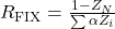 | | Converting floating-rate debt to fixed-rate liabilities |
| Currency Swaps | 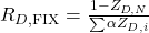 | ![V_{\text{swap},D} = B_D(t) - [B_F(t) \cdot S_t(D/F)]](https://www.SuperBusinessManager.com/wp-content/ql-cache/quicklatex.com-7747a897f68b3a12a60228d0485a1413_l3.png "Rendered by QuickLaTeX.com") | Multicurrency capital structure optimization |
| Equity Swaps | |  | Synthetic index tracking, tax-efficient rebalancing |
Conclusion: Strategic Recommendations for Executive Leadership
The Pricing and Valuation of Forward Commitments provides an indispensable framework for navigating complex global financial markets. By understanding the carry arbitrage model, zero-coupon yield curve structures, and mark-to-market valuation dynamics, financial executives can effectively insulate their organizations against adverse movements in equity prices, interest rates, bond yields, and foreign currencies.
Chief Executive Officers, Chief Financial Officers, and Corporate Treasurers should implement the following strategic measures:
- Establish Integrated Valuation Systems: Deploy robust quantitative pricing architecture to perform real-time mark-to-market valuations and scenario stress testing across all outstanding forward commitments.
- Monitor Carry Costs and Yield Curves: Continuously audit intermediate cashflows, continuous yields, storage expenses, and interest rate term structures to capture mispricing opportunities and mitigate collateral margin call risks.
- Optimize Collateral Management: Align exchange-traded futures margin requirements and over-the-counter ISDA collateral framework thresholds to preserve liquidity during volatile market cycles.
- Maintain Strict Treasury Governance: Enforce clear counterparty credit limits and independent quantitative reviews to verify derivative pricing, preventing unhedged financial losses and maximizing risk-adjusted enterprise value.
