In the architecture of global capital markets, the precise calculation, comparison, and interpretation of financial returns serve as the cornerstone of portfolio management and asset allocation. Institutional investors, corporate treasurers, and financial analysts rely on robust mathematical frameworks to evaluate the historical performance of diverse financial assets, instruments, and economic indicators.
Without standardized quantitative methodologies, comparing the performance of a high-yield corporate bond against a global equity index or assessing the erosion of purchasing power from macroeconomic inflation indicators becomes impossible.
This article examines the core mathematical formulations of financial returns, provides concrete calculations to illustrate their mechanics, and analyzes their comparative applications across global markets.
Mathematical Frameworks and Return Calculations
To evaluate investment performance accurately, financial professionals deploy several distinct mathematical models. Each model addresses specific valuation challenges, including cash flow timing, multi-period compounding, and volatility drag.
1. Holding Period Return
The Holding Period Return measures the total percentage return earned from an asset over a specific investment horizon, combining capital appreciation with income distributions such as dividends or coupon payments.
Consider an investor who purchases shares of a multinational corporation at an initial price of  . Over a one-year holding period, the stock distributes a total dividend of
  and ends the period at an ending price of
  . The Holding Period Return is calculated using the formula:
![\[HPR = \frac{(P_1 - P_0) + D_1}{P_0}\]](https://www.SuperBusinessManager.com/wp-content/ql-cache/quicklatex.com-30c70faf38d4c8b6a0af34303e214c54_l3.png "Rendered by QuickLaTeX.com")
Substituting the values:
![\[HPR = \frac{(115.00 - 100.00) + 3.00}{100.00} = \frac{15.00 + 3.00}{100.00} = \frac{18.00}{100.00} = 0.18 \text{ or } 18.00\%\]](https://www.SuperBusinessManager.com/wp-content/ql-cache/quicklatex.com-38375c3d9952883391ea4c06a9bef6cf_l3.png "Rendered by QuickLaTeX.com")
2. Arithmetic Versus Geometric Mean Returns
When evaluating multi-period performance, analysts must distinguish between the arithmetic mean and the geometric mean. The arithmetic mean calculates the simple average of periodic returns, whereas the geometric mean calculates the compound annual growth rate, capturing the critical impact of volatility drag.
Suppose an equity portfolio experiences a return of  in year one and
  in year two.
The arithmetic mean return is calculated as:
![\[R_{\text{arithmetic}} = \frac{R_1 + R_2}{2} = \frac{0.20 + (-0.20)}{2} = 0.00 \text{ or } 0.00\%\]](https://www.SuperBusinessManager.com/wp-content/ql-cache/quicklatex.com-4cf5bda8d0cc3cf6919b95bff07d6cf5_l3.png "Rendered by QuickLaTeX.com")
However, the true terminal value of a USD100,000 portfolio after two years tells a different story. After year one, the portfolio value rises to USD120,000. After year two, a  decline reduces the value to USD120,000 x (1 – 0.20) = USD96,000.
The geometric mean return accounts for this compounding reality:
![\[R_{\text{geometric}} = \sqrt{(1 + R_1) \times (1 + R_2)} - 1\]](https://www.SuperBusinessManager.com/wp-content/ql-cache/quicklatex.com-d54019daff7a406d39fe9ae5a0dc3178_l3.png "Rendered by QuickLaTeX.com")
Substituting the values:
![\[R_{\text{geometric}} = \sqrt{(1 + 0.20) \times (1 - 0.20)} - 1 = \sqrt{1.20 \times 0.80} - 1 = \sqrt{0.96} - 1 \approx 0.9798 - 1 = -0.0202 \text{ or } -2.02\%\]](https://www.SuperBusinessManager.com/wp-content/ql-cache/quicklatex.com-9ee33e545c863560c949dda643f72c3b_l3.png "Rendered by QuickLaTeX.com")
This calculation demonstrates that over multi-year horizons, the geometric mean provides an accurate reflection of wealth accumulation, highlighting how volatility reduces terminal wealth even when the arithmetic average appears neutral.
3. Money-Weighted Versus Time-Weighted Returns
To evaluate portfolio manager performance versus client cash flow decisions, analysts utilize Money-Weighted and Time-Weighted returns.
The Money-Weighted Return represents the Internal Rate of Return (IRR) of a portfolio, equating the present value of all cash inflows (initial investments and capital additions) to the present value of all cash outflows (withdrawals and ending portfolio value). MWR is heavily influenced by the size and timing of external cash flows controlled by the investor.
Conversely, the Time-Weighted Return compounds the returns of sub-periods, effectively neutralizing the distorting impact of external cash flows. TWR measures the compound rate of growth of a single unit of currency invested in the portfolio, making it the industry standard for evaluating the pure investment skill of a portfolio manager.
In the governance of institutional asset management, evaluating portfolio performance requires distinguishing between the investment skill of the portfolio manager and the impact of client-driven capital allocation decisions. Two primary metrics govern this evaluation: the Time-Weighted Return and the Money-Weighted Return. While the time-weighted return isolates managerial efficacy by neutralizing external cash flows, the money-weighted return calculates the internal rate of return, accounting for the exact magnitude and timing of all capital contributions and withdrawals.
Understanding the mathematical mechanics and divergence between these two metrics is essential for institutional investors, corporate treasurers, and wealth managers. This article provides a comprehensive, step-by-step calculation and comparative interpretation of Money-Weighted and Time-Weighted Returns using a concrete multi-period financial scenario.
Scenario Parameters and Cash Flow Timeline
To illustrate the distinct calculations of Money-Weighted and Time-Weighted Returns, consider a two-year investment portfolio with the following transactional history:
- Initial Outlay (
 ): An institutional investor commits an initial capital allocation of
  to a global equity strategy.
 - End of Year 1 (
 (Before Cash Flow)): Due to strong market performance, the portfolio value grows to
  prior to any transactions.
 - Year 1 Cash Flow ( (Transaction)): Recognizing positive momentum, the institutional investor adds an additional capital injection of
 , bringing the total capital base to
  .
. - End of Year 2 (
 ): At the conclusion of the second year, the total portfolio value reaches
  , at which point the portfolio is liquidated.
Calculating the Time-Weighted Return
The Time-Weighted Return measures the compound rate of growth of a single unit of currency invested in the portfolio over a measurement period. It eliminates the distorting effects of external cash inflows and outflows, making it the industry benchmark for evaluating portfolio manager skill.
Step 1: Divide the Investment Horizon into Sub-Periods
The investment timeline is divided into distinct sub-periods bounded by external cash flows:
- Sub-Period 1 ( to ): Spans from the initial investment to the cash injection at year one.
- Sub-Period 2 ( to ): Spans from the post-injection capital base to the final liquidation at year two.
Step 2: Calculate Sub-Period Returns
For Sub-Period 1, the return ( ) is calculated using the initial value and the portfolio value immediately before the cash flow:
![\[R_1 = \frac{\$1,200,000 - \$1,000,000}{\$1,000,000} = \frac{\$200,000}{\$1,000,000} = 0.20 \text{ or } 20.00\%\]](https://www.SuperBusinessManager.com/wp-content/ql-cache/quicklatex.com-862fa70e75ed3c19c1e06d5fa6e29edd_l3.png "Rendered by QuickLaTeX.com")
For Sub-Period 2, the return ( ) is calculated using the starting portfolio base after the cash injection (1,200,000 + 500,000 = 1,700,000) and the ending portfolio value (1,800,000):
![\[R_2 = \frac{\$1,800,000 - \$1,700,000}{\$1,700,000} = \frac{\$100,000}{\$1,700,000} \approx 0.0588 \text{ or } 5.88\%\]](https://www.SuperBusinessManager.com/wp-content/ql-cache/quicklatex.com-e4ecdec313458b8d2fa6a8922e015030_l3.png "Rendered by QuickLaTeX.com")
Step 3: Compound the Sub-Period Returns
To determine the cumulative Time-Weighted Return ( ), the sub-period growth factors are compounded together:
![\[1 + TWR_{\text{cumulative}} = (1 + R_1) \times (1 + R_2)\]](https://www.SuperBusinessManager.com/wp-content/ql-cache/quicklatex.com-e6927138e33e2923000cf05e0d4464df_l3.png "Rendered by QuickLaTeX.com")
![\[1 + TWR_{\text{cumulative}} = (1 + 0.20) \times (1 + 0.0588) = 1.20 \times 1.0588 = 1.27056\]](https://www.SuperBusinessManager.com/wp-content/ql-cache/quicklatex.com-618c60fe67b53d9fe63344a41fc01846_l3.png "Rendered by QuickLaTeX.com")
![\[TWR_{\text{cumulative}} = 1.27056 - 1 = 0.27056 \text{ or } 27.06\%\]](https://www.SuperBusinessManager.com/wp-content/ql-cache/quicklatex.com-75a305e90bee471c4699603a30ae3c76_l3.png "Rendered by QuickLaTeX.com")
To express this on an annualized geometric mean basis over the two-year period:
![\[TWR_{\text{annualized}} = \sqrt{1.27056} - 1 \approx 1.1272 - 1 = 0.1272 \text{ or } 12.72\%\]](https://www.SuperBusinessManager.com/wp-content/ql-cache/quicklatex.com-ac6503096c4fb944a1b64723a84186de_l3.png "Rendered by QuickLaTeX.com")
Calculating the Money-Weighted Return
The Money-Weighted Return equates the present value of all cash inflows to the present value of all cash outflows, functioning identically to the Internal Rate of Return (IRR). It reflects the exact growth experienced by the investor’s capital, factoring in the timing of contributions.
Step 1: Establish the Cash Flow Equation
The cash flows associated with the investor are:
 (initial cash outflow from investor)
 (additional cash outflow from investor at year one)
 (cash inflow to investor at year two liquidation)
The internal rate of return equation sets the net present value of these cash flows to zero, where  represents the Money-Weighted Return:
![\[0 = CF_0 + \frac{CF_1}{(1 + r)^1} + \frac{CF_2}{(1 + r)^2}\]](https://www.SuperBusinessManager.com/wp-content/ql-cache/quicklatex.com-a172aa258b1060635b06a4914d76e462_l3.png "Rendered by QuickLaTeX.com")
![\[0 = -1,000,000 - \frac{500,000}{1 + r} + \frac{1,800,000}{(1 + r)^2}\]](https://www.SuperBusinessManager.com/wp-content/ql-cache/quicklatex.com-6029e6c0e83112223c388f8817b9c91c_l3.png "Rendered by QuickLaTeX.com")
Step 2: Solve for the Internal Rate of Return
To solve this quadratic equation, substitute  :
:
![\[1,800,000x^2 - 500,000x - 1,000,000 = 0\]](https://www.SuperBusinessManager.com/wp-content/ql-cache/quicklatex.com-9259b032a5d74e588cd7200030fbf4fe_l3.png "Rendered by QuickLaTeX.com")
Dividing the entire equation by  simplifies the expression:
![\[18x^2 - 5x - 10 = 0\]](https://www.SuperBusinessManager.com/wp-content/ql-cache/quicklatex.com-fa51d7193f605d3f4cc09e3392038849_l3.png "Rendered by QuickLaTeX.com")
Applying the quadratic formula 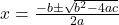 :
:
![\[x = \frac{-(-5) \pm \sqrt{(-5)^2 - 4(18)(-10)}}{2(18)}\]](https://www.SuperBusinessManager.com/wp-content/ql-cache/quicklatex.com-46f24ab4656e6ee31aadc952cd5d5d7f_l3.png "Rendered by QuickLaTeX.com")
![\[x = \frac{5 \pm \sqrt{25 + 720}}{36} = \frac{5 \pm \sqrt{745}}{36}\]](https://www.SuperBusinessManager.com/wp-content/ql-cache/quicklatex.com-4e569aa69c7df08bc4e4935d92b661cd_l3.png "Rendered by QuickLaTeX.com")
Calculating the square root of  (approximately
  ):
):
![\[x = \frac{5 + 27.2947}{36} = \frac{32.2947}{36} \approx 0.897075\]](https://www.SuperBusinessManager.com/wp-content/ql-cache/quicklatex.com-786adc15fa65bc5b02eac7ab1df12e57_l3.png "Rendered by QuickLaTeX.com")
Since , we isolate  :
:
![\[1 + r = \frac{1}{0.897075} \approx 1.11473\]](https://www.SuperBusinessManager.com/wp-content/ql-cache/quicklatex.com-5a5606054b24420578e546f87267d53a_l3.png "Rendered by QuickLaTeX.com")
![\[r = 1.11473 - 1 = 0.11473 \text{ or } 11.47\%\]](https://www.SuperBusinessManager.com/wp-content/ql-cache/quicklatex.com-4f6fae8541b80e4ec13f3a58a2d9b3b4_l3.png "Rendered by QuickLaTeX.com")
Thus, the Money-Weighted Return is 11.47%.
Comparative Analysis and Interpretation
A direct comparison of our calculations reveals a notable divergence:
| Return Metric | Calculated Performance | Primary Evaluative Focus |
| Time-Weighted Return (Annualized) | 12.72% | Evaluates portfolio manager investment skill |
| Money-Weighted Return (IRR) | 11.47% | Evaluates actual investor wealth accumulation |
Interpreting the Discrepancy
The Time-Weighted Return ( ) exceeds the Money-Weighted Return (
 ). This divergence occurs because of cash flow timing.
The portfolio generated an exceptional return of in the first sub-period, driven by the initial . However, the investor injected an additional at , after this surge had already occurred. In the second sub-period, the expanded capital base earned a much lower return of only  . Because the investor committed a larger volume of capital just before a period of lower performance, the investor’s realized internal rate of return was penalized relative to the manager’s pure asset-level performance.
Comparative Analysis of Asset Classes and Indicators
Comparing returns across different asset classes requires standardizing metrics to account for distinct cash flow structures, liquidity profiles, and risk characteristics. Financial indicators, such as inflation rates or currency exchange movements, further require careful interpretation.
| Asset Class or Indicator | Primary Return Metric | Sample Calculation Parameter | Main Analytical Objective |
| Corporate Equities | Geometric Mean / Time-Weighted | Capital gains plus dividend yield over multi-year horizons | Measure long-term wealth accumulation and managerial alpha |
| Fixed Income Instruments | Yield-to-Maturity / Current Yield | Annual coupon payment divided by current market price | Evaluate contractual income and capital preservation |
| Real Estate Assets | Total Return (Cap Rate plus Growth) | Net operating income divided by property value plus appreciation | Assess rental yield and capital appreciation |
| Macroeconomic Indicators | Percentage Change (Inflation Rate) | Price index year-over-year percentage difference | Gauge purchasing power erosion and economic cost pressures |
When interpreting these comparative metrics, analysts must evaluate the underlying economic drivers. For instance, fixed-income returns are primarily anchored by contractual interest payments and interest rate sensitivity, whereas equity returns are driven by corporate earnings growth and multiple expansion. Comparing these figures directly requires adjusting for risk profiles and holding durations.
Global Business Implementation and Case Studies
Applying return calculations in real-world environments demonstrates how these methodologies operate across diverse market sectors and geographic regions.
Consider the historical multi-year performance evaluation of multinational corporations listed on international exchanges, such as Tokyo-listed Toyota Motor Corporation or London-listed Shell PLC. When institutional asset managers evaluate these equities, they compute multi-period holding period returns and geometric mean growth rates over five-year horizons. This approach smooths out interim macroeconomic shocks, commodity price fluctuations, and currency volatility, providing a clear picture of fundamental enterprise value creation.
Another prominent example involves cross-border fixed-income instruments, such as the euro-denominated green bonds issued by the European Investment Bank. Institutional fixed-income analysts calculate the yield-to-maturity by determining the internal rate of return that equates the current bond price to the present value of all future coupon payments and principal repayment. When foreign investors purchase these euro-denominated instruments, they calculate holding period returns inclusive of currency translation effects against their domestic currency, utilizing time-weighted methodologies to isolate underlying credit performance from currency fluctuations.
Conclusions
The accurate calculation, comparison, and interpretation of financial returns are indispensable skills for modern financial analysis. By mastering quantitative formulas ranging from basic holding period returns to complex geometric compounding and internal rate of return models, market participants can successfully evaluate diverse asset classes, instruments, and macroeconomic indicators. Understanding the nuances of these return metrics ensures that capital is deployed efficiently, risks are properly priced, and strategic investment decisions are executed effectively in an increasingly complex global economy.
